Device Fabrication Concepts

A quantum-material device is not a pristine Hamiltonian with wires attached afterward. Patterning changes boundaries; contacts exchange charge and broaden states; gates create electric fields and trap dynamics; dielectrics screen interactions; transfer creates strain and interfaces; etching creates edges and defects; packaging sets thermal, electromagnetic, and mechanical boundary conditions. Fabrication is therefore part of the physical preparation of the system.

The aim is to understand how fabrication changes the system you measure: why a longer contact may stop helping, why a gate voltage may not give the expected carrier density, and why a cold refrigerator need not contain cold electrons. Material-specific cleanroom recipes are outside this discussion. For the connection between device variation and qubit performance, see Materials and Fabrication Interface.

Required background. How Quantum Matter Is Measured explains how calibration connects an instrument reading to a physical quantity. Transport Measurements supplies contact, geometry and readout checks. van der Waals Heterostructures supplies the layer, interface and alignment choices whose physical effects must be controlled during assembly.

How fabrication changes a quantum system

A contact can dope the channel, a dielectric can change interaction strengths, and an etch can alter both confinement and scattering. These changes must be included when choosing a model.

A schematic low-energy decomposition is

$$H_{\mathrm{device}}=H_{\mathrm{material}}+H_{\mathrm{confinement}} +H_{\mathrm{electrostatic}}+H_{\mathrm{contact}}+H_{\mathrm{strain}} +H_{\mathrm{disorder}}+H_{\mathrm{environment}}.$$

The terms need not be separately measurable or even sharply separable. The decomposition reminds us to include the effects of apparently passive components. A metal contact can contribute electrostatic doping, hybridization, strain, screening, spin–orbit coupling, exchange, superconducting pairing, and dissipation at once.

A device cross-section should identify:

• active material, thickness, composition, crystal axes, and relevant surfaces or edges;
• substrate, buffer, encapsulant, spacer, dielectric, and adhesion layers;
• contact material, geometry, overlap, interface preparation, and lead routing;
• local and global gates, dielectric thicknesses, and grounded conductors;
• patterned dimensions and the metrology method defining them;
• expected current paths, voltage probes, leakage paths, and capacitive couplings;
• thermal anchors, filters, radiation shields, and mechanical constraints.

Use “nominal” for a mask or deposition target and “measured” for a post-process dimension. Sidewall angle, overetch, undercut, redeposition, line-edge roughness, film stress, and grain structure can make the two differ.

Relating a process change to a physical change

Growth, transfer, lithography, etching, deposition, annealing, and packaging can each change several properties at once. For example, an anneal that lowers contact resistance may also move impurities or relax strain. Measure the relevant property before and after the change, and use a nearby witness sample or an otherwise comparable untreated device to identify its cause.

Keep the sample identity, material lot, actual treatment conditions, exposure history, and measured dimensions with the electrical data. These details make it possible to compare devices made on different days without confusing a process change with a different starting crystal.

Contacts

A contact is a reservoir and an interface

An electrical contact should be specified by what it must do. It may need to inject equilibrium carriers, sense voltage with negligible current, define a tunnel barrier, preserve spin or valley polarization, induce superconductivity, transmit microwaves, or remain noninvasive to a fragile state. “Low resistance” is not sufficient for all of these tasks.

At a metal–semiconductor interface, work-function mismatch, interface dipoles, surface states, chemical bonding, and electrostatic screening determine band bending and carrier injection. The elementary Schottky–Mott picture is often modified by Fermi-level pinning; Sze and Ng develop these semiconductor-interface models. At a metal–two-dimensional-material interface, top contacts, edge contacts, residues, damage, and metal-induced doping produce distinct boundary conditions. At a normal–superconductor interface, transparency and disorder determine whether the contact acts as an ordinary reservoir, tunnel probe, or proximity source.

Useful contact observables include:

• two- and four-terminal resistance versus temperature, gate, bias, and field;
• contact linearity and symmetry in current–voltage curves;
• transfer-length or multiple-length structures;
• stability under thermal cycles and current stress;
• noise, drift, telegraph switching, and electromigration;
• spectroscopic evidence for a tunnel barrier or induced gap;
• spatial evidence for contact doping, reaction, or delamination.

An apparently linear $I$–$V$ curve over one bias window does not prove an ohmic microscopic interface. Thermal broadening, parallel conduction, or an overly narrow window can hide a barrier.

Why current crowds near a contact edge

A length series can separate contact and channel contributions. For a diffusive, uniform channel of width $W$, identical contacts, and negligible lead resistance,

$$R_{2\mathrm t}(L)=2R_c+R_{\mathrm{ch}}\frac{L}{W}.$$

Here $L$ is the edge-to-edge channel length, $R_{\mathrm{ch}}$ is its sheet resistance, and $R_c$ is the resistance of one contact. The intercept determines $2R_c$; the slope determines $R_{\mathrm{ch}}/W$. Nonuniform doping, different contacts, dimensional errors, or ballistic transport can spoil this interpretation. Schroder describes these measurement methods.

To see why contact area alone is insufficient, consider the transmission-line model discussed by Berger. An equipotential metal covers a resistive sheet for $0<x<L_c$, with $x=0$ at the channel edge. Let $R_u$ be the sheet resistance under the contact, and let $\rho_c$ be a uniform specific interface resistivity, in $\Omega\,\mathrm{m^2}$. They need not equal the channel’s properties.

If $v(x)$ is the sheet potential relative to the metal, the current $I(x)$ flowing into the overlap obeys

$$\frac{dv}{dx}=-\frac{R_u}{W}I, \qquad \frac{dI}{dx}=-\frac{W}{\rho_c}v.$$

The second equation says that current leaves the sheet vertically through the interface. Combining them gives $v''=v/L_T^2$, where

$$L_T=\sqrt{\frac{\rho_c}{R_u}}.$$

No lateral current exits the far end: $I(L_c)=0$. With $v(0)=v_e$, the solution is

$$v(x)=v_e\frac{\cosh[(L_c-x)/L_T]}{\cosh(L_c/L_T)}.$$

Therefore

$$R_cW=\frac{v_eW}{I(0)} =\sqrt{\rho_cR_u}\,\coth(L_c/L_T).$$

For $L_c\ll L_T$, nearly the entire contact carries vertical current and $R_c\simeq\rho_c/(WL_c)$. For $L_c\gg L_T$, most current transfers within a few $L_T$ of the channel edge; increasing the overlap then gives little improvement.

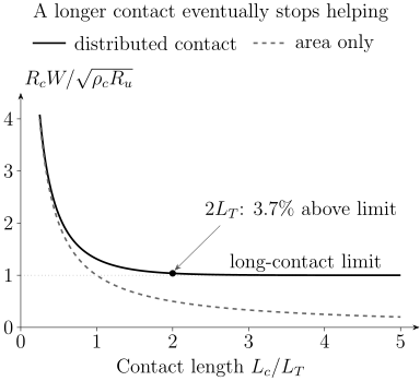
The transmission-line prediction is $R_cW/\sqrt{\rho_cR_u}=\coth(L_c/L_T)$. The dashed area-only estimate $L_T/L_c$ works for a short contact but misses the saturation. At $L_c=2L_T$, the resistance is already within about $3.7\%$ of its long-contact limit.

The length-series slope measures $R_{\mathrm{ch}}$, not $R_u$. Inferring $\rho_c$ from the intercept requires separate knowledge of $R_u$, or a justified approximation $R_u\simeq R_{\mathrm{ch}}$. Contact-induced doping is one reason they differ. The model also assumes local ohmic conduction, a thin uniform sheet and negligible metal resistance; coherent channels, superconducting interfaces, and edge contacts need appropriate alternatives.

Contacts can be invasive

A voltage probe is noninvasive only when the current it draws and the equilibration it causes are negligible for the intended observable. In a coherent conductor, a contact can absorb phase information and redistribute populations. In a two-dimensional channel, the metal can screen gates and alter density beneath the overlap. In a small island, the contact capacitance and tunnel rate become terms in the Hamiltonian.

Compare contact resistance at the actual temperature, gate voltage, and bias used in the experiment. Record the interface preparation and overlap dimensions, because an apparently identical metal can produce a different interface after an air exposure or cleaning step. Allain and colleagues discuss semiconductor contacts; Wang and colleagues demonstrate an edge-contact geometry.

Conductance Quantization explains coherent channel and reservoir resistance. Proximity and Andreev Physics treats superconducting-interface scattering; Superconducting Proximity Effect develops spatial pair correlations and inverse proximity.

Gates and electrostatics

Geometric capacitance is the first approximation

For a parallel-plate dielectric of thickness $d$ and relative permittivity $\epsilon_r$, the geometric capacitance per area is

$$c_{\mathrm{geo}} = \frac{\epsilon_0\epsilon_r}{d}.$$

Let $n_s$ denote the added electron density relative to a reference state, with $e>0$. For a uniform channel connected to an electron reservoir, negligible chemical-potential change and negligible trapped charge give

$$en_s = c_{\mathrm{geo}} \left( V_g-V_0 \right).$$

$V_0$ absorbs built-in potentials and fixed charge. This conversion fails when quantum capacitance, trap charging, fringing fields, multiple conductors, depletion, dielectric nonlinearity, or mobile ions matter.

Adding electrons also changes their chemical potential $\mu$. In quasistatic equilibrium with the reservoir,

$$\Delta V_g=\frac{en_s}{c_{\mathrm{geo}}}+\frac{\Delta\mu}{e}.$$

The first term charges the dielectric; the second changes the electron system. Differentiating at fixed temperature and other control parameters gives the thermodynamic quantum capacitance and measured differential capacitance per area:

$$c_Q=e^2\left(\frac{\partial n_s}{\partial\mu}\right)_T, \qquad c_{\mathrm{eff}}=e\frac{\partial n_s}{\partial V_g},$$ $$\frac{1}{c_{\mathrm{eff}}} =\frac{1}{c_{\mathrm{geo}}}+\frac{1}{c_Q}.$$

For a positive $c_Q$ smaller than $c_{\mathrm{geo}}$, much of the gate-voltage change raises $\mu$. This is a local slope, not generally a constant conversion factor over a large sweep: integrate $c_{\mathrm{eff}}(V_g)/e$ to obtain a density change. The single-particle density of states gives $c_Q$ only when the corresponding noninteracting approximation applies. Interactions can produce negative electronic compressibility and $c_{\mathrm{eff}}>c_{\mathrm{geo}}$, as in the measurements by Li and colleagues. In this uniform model, stability still requires the total inverse capacitance to be positive.

Trap charging adds frequency and history dependence. The relation above assumes traps are absent or frozen with a fixed offset, and that carriers can equilibrate through the contacts during the measurement. A low measured ac capacitance can also result from slow resistive charging rather than a small equilibrium compressibility.

Multiple gates require a capacitance matrix

For fixed linear dielectrics, a useful electrostatic convention is

$$q_i-q_i^{(0)}=\sum_{j\ne i}c_{ij}(V_i-V_j),$$

where $c_{ij}=c_{ji}\ge0$ are mutual capacitances and the reference conductor is included among the $j$. These coefficients differ from the off-diagonal entries of the Maxwell capacitance matrix, which have the opposite sign. Fixed charge is represented by $q_i^{(0)}$; changing trap populations cannot be absorbed into one fixed offset.

Local gates usually affect several device parameters. A virtual-gate transformation uses a measured response Jacobian to choose voltage combinations that tune selected parameters approximately independently. This requires enough independent controls; a rank-deficient response cannot be inverted, and a poorly conditioned response amplifies calibration errors. The transformation is local and can drift when traps switch.

For a simple dual-gated layer in the large-$c_Q$, parallel-plate approximation, one common convention is

$$\begin{aligned} en_s &= c_t\Delta V_t + c_b\Delta V_b, \\ D_z &= \frac{1}{2} \left( c_t\Delta V_t - c_b\Delta V_b \right). \end{aligned}$$

$D_z$ here is a gate-defined displacement coordinate with units of charge per area, not automatically the microscopic field inside the layer; some literature divides it by $\epsilon_0$ or reverses its sign. State the convention. The offset voltages $\Delta V_t$ and $\Delta V_b$ should be calibrated from charge-neutrality, quantum Hall, compressibility, or another measured feature rather than assumed from zero instrument voltage.

Gate quality is multidimensional

A gate stack should be tested for:

• leakage current and its temperature, field, polarity, and sweep-rate dependence;
• dielectric breakdown and soft pre-breakdown damage;
• hysteresis, relaxation, and charge jumps;
• cross-capacitance to contacts and neighboring gates;
• spatial nonuniformity and fringe-field confinement;
• dielectric loss and microwave heating;
• displacement-current artifacts during sweeps;
• stability across cooldowns and illumination history.

The average electric field $|V|/d$ is only a screening estimate. Local fields concentrate at edges, particulates, pinholes, thickness steps, and sharp metal corners. A device operated once near nominal breakdown may be permanently changed even if it does not short.

Heterostructure assembly

Nominal sequence is not local structure

Layered devices can be grown directly, wafer-bonded, transferred, picked up, stamped, laminated, or assembled through combinations of these methods. The durable requirements are to know:

• layer identity, thickness, polytype, and orientation before assembly;
• sequence, overlap area, intended registry, and exposed interfaces;
• temperature, atmosphere, pressure, and residence time relevant to adhesion or reaction;
• local twist, strain, bubbles, wrinkles, tears, folds, and trapped contamination afterward;
• whether later lithography, etching, or annealing changed the buried interface.

In rotationally sensitive systems, the fabrication angle is a target, not the final local twist field. Elastic relaxation and heterostrain can create domains and spatially varying moiré periods. Structural and spectroscopic metrology should therefore be linked to the actual transport or optical region.

Frisenda and colleagues review assembly methods, and Pizzocchero and colleagues describe hot pickup. For the physical consequences, see van der Waals Heterostructures and Moiré Superlattices: the local angle and strain determine the electronic scales, even when the nominal assembly angle is unchanged.

Selection begins before measurement

Selecting large flakes, flat regions and working contacts may be sensible, but it changes the population eventually measured. Let $A_j$ mean that a candidate passes stage $j$. The fraction that passes every stage follows the probability chain rule:

$$Y_{\mathrm{total}} =P(A_1)\prod_{j=2}^{m}P(A_j\mid A_1,\ldots,A_{j-1}).$$

No independence assumption is needed when each factor is conditional on all earlier passes. Multiplying separately measured marginal yields generally fails: a thick flake may survive transfer well but be difficult to gate. Count the same starting cohort through assembly, patterning, contacting and cooldown, and distinguish physical failures from devices simply not selected for further study.

Encapsulation

Encapsulation can isolate an active material from oxygen, water, polymers, adsorbates, ion motion, mechanical abrasion, and direct lithographic exposure. It can also provide an atomically flatter dielectric environment and enable edge contacts. For air-sensitive materials, the atmosphere and time between exfoliation, assembly, and sealing can determine whether the intended phase survives at all.

Encapsulation is not physically neutral. It changes:

• dielectric screening and therefore Coulomb interactions and exciton binding;
• electrostatic disorder and gate capacitance;
• strain, thermal contraction, pressure, and wrinkle formation;
• heat flow and optical interference;
• surface phonons and remote scattering;
• chemical potential through trapped charge or residues;
• access for scanning probes, adsorbates, or local gates.

The substrate and encapsulant must therefore be characterized as parts of the device. Dean and colleagues demonstrate the benefits of a boron-nitride environment for graphene. Those benefits do not imply that every encapsulated interface is residue-free: record the layer thicknesses, exposed edges, assembly atmosphere and aging behavior alongside local microscopy or spectroscopy.

Cleanliness and process-induced disorder

Clean means fit for an observable

No single cleanliness metric covers every experiment. A surface can be sufficiently free of charged disorder for high mobility yet unsuitable for scanning tunneling because of sparse adsorbates. A tunnel junction can be electrically uniform while containing enough magnetic defects to broaden a spin-sensitive spectrum. A contact can be low resistance but chemically react with the active layer.

Common process-induced perturbations include:

Source	Possible device term	Useful control
polymer or solvent residue	doping, traps, tunnel barrier, adsorbate scattering	witness surface, AFM, spectroscopy, alternate resist or protected interface
plasma or ion damage	vacancies, edge disorder, amorphization, implanted charge	dose split, Raman or microscopy, protected control region
etch redeposition	leakage path, edge doping, contact barrier	cross-section, sidewall inspection, electrical isolation test
metal diffusion or reaction	alloyed contact, gap states, magnetic or superconducting proximity	composition depth profile, temperature-budget split
trapped interface contamination	bubbles, local strain, dielectric gaps	optical, AFM, Raman, local transport or scanning probe
dielectric charge traps	hysteresis, drift, telegraph noise, density puddles	sweep-rate, time, temperature, frequency, illumination tests
film stress and thermal mismatch	strain, cracks, delamination, symmetry change	wafer curvature, Raman, diffraction, cooldown cycling
particulate or pinhole	local field concentration, gate leakage, shorts	dark-field inspection, leakage maps, breakdown statistics

Cleaning and annealing are interventions, not erasers. They may remove one residue while mobilizing another contaminant, reacting a contact, changing stoichiometry, relaxing twist, creating vacancies, or increasing diffusion. Compare a suitable observable before and after treatment, with a compatible control. Pirkle and colleagues provide an example of transfer residues changing graphene properties.

Mobility is not a purity certificate

In a simple band,

$$\mu = \frac{e\tau_{\mathrm{tr}}}{m^\ast}.$$

The transport lifetime $\tau_{\mathrm{tr}}$ weights momentum relaxation. Quantum oscillation or spectroscopic linewidths can instead constrain a single-particle lifetime $\tau_q$, which weights scattering differently. Smooth disorder can give a large $\tau_{\mathrm{tr}}/\tau_q$ ratio, while rare strong defects may dominate local behavior without greatly changing average mobility.

Characterize disorder at the scale relevant to the claim:

• composition and crystallinity for bulk or epitaxial defects;
• surface and interface topography for roughness and bubbles;
• Raman, optical, or diffraction maps for strain and domains;
• density inhomogeneity and compressibility for electrostatic puddles;
• low-frequency noise for active traps;
• transport and quantum lifetimes for angular scattering;
• device-to-device distributions for process variability.

Disorder in Quantum Matter explains the statistical classification and physical consequences of these perturbations.

Cryogenic measurement environment

The electron temperature must be demonstrated

The refrigerator’s thermometer measures a location in the cryostat, not necessarily the electronic distribution in the device. Joule power in a resistive element is

$$P = IV = I^2R = \frac{V^2}{R}$$

for a lumped linear resistor with the voltage across that element. The source power is not necessarily deposited in the active channel: ballistic conductors can dissipate much of it in their reservoirs. If electron–electron relaxation establishes a local thermal distribution, a common electron–phonon cooling model is

$$P_{\mathrm{e-ph}} = \Sigma\mathcal V \left( T_e^p-T_{\mathrm{ph}}^p \right),$$

so a steady state gives

$$T_e = \left( T_{\mathrm{ph}}^p + \frac{P}{\Sigma\mathcal V} \right)^{1/p}.$$

$\Sigma$, volume $\mathcal V$, and exponent $p$ depend on material, dimensionality, disorder, and temperature range. The expression is a diagnostic model, not a universal thermometer. Contact cooling, photon exchange and substrate heating may dominate; a nonthermal electronic distribution may have no single $T_e$. Wellstood and colleagues study hot-electron effects in metals, while Pobell discusses low-temperature thermalization more broadly.

Demonstrate electronic temperature with a calibrated noise, Coulomb-blockade, quantum-dot, superconducting, or other primary or secondary thermometer near the active device when low-energy claims depend on it. Excitation-amplitude extrapolation and dwell-time tests help separate saturation from intrinsic behavior.

Wiring defines bandwidth and noise

An ideal voltage source driving a series resistance $R$ and a shunt capacitance $C$, with negligible output loading, gives a low-pass cutoff

$$f_c = \frac{1}{2\pi RC}.$$

At frequencies $hf\ll k_BT$, a resistor’s one-sided open-circuit Johnson voltage-noise density is

$$S_V(f) = 4k_BTR.$$

Real cryogenic lines contain distributed capacitance and inductance, thermoelectric junctions, dielectric loss, resonances, ground loops, amplifier backaction, triboelectric noise, and radio-frequency leakage. Filtering trades bandwidth and settling time against noise and heating. A nominal lock-in frequency can still mix with line resonances or gate displacement currents.

A cryogenic integration record should include:

• wire material, gauge, routing, shielding, and thermal anchors at each stage;
• room-temperature and cryogenic filters, attenuation, cutoff, and measured transfer function;
• source and detector impedances, compliance, input bias, and grounding;
• sample mount, connector, bond-wire, and contact configuration;
• thermometer location, thermalization evidence, and excitation-power sweep;
• magnetic materials, trapped-flux procedure, vector alignment, and field-dependent heating;
• illumination, radiation shielding, vacuum, pressure medium, and thermal-cycle history.

Thermal contraction can strain a thin crystal or break a marginal contact. Magnetic field can heat metallic parts through eddy currents during a sweep. Gate lines can carry radio-frequency noise directly to a small electron system. Packaging is therefore the final fabrication step.

Reproducibility

Preserve the hierarchy

Measurements are nested: repeated sweeps belong to one cooldown; cooldowns belong to one device; devices belong to one chip, flake, wafer region, or stack; those belong to a fabrication batch and source material. Repeated sweeps do not substitute for independent devices.

A simple variance-components model is

$$y_{bdr} = \mu + \beta_b + \delta_{bd} + \epsilon_{bdr},$$

where $\beta_b$ is a batch effect, $\delta_{bd}$ a device-within-batch effect, and $\epsilon_{bdr}$ repeat-level variation. Suppose these effects are independent, centered, and have variances $\sigma_b^2$, $\sigma_d^2$ and $\sigma_r^2$. For a balanced sample with $B$ batches, $D$ devices per batch and $R$ repeats per device,

$$\operatorname{Var}(\bar y) =\frac{\sigma_b^2}{B} +\frac{\sigma_d^2}{BD} +\frac{\sigma_r^2}{BDR}.$$

More sweeps reduce only the last term. More devices in the same batch do not remove uncertainty from batch variation. Even without enough batches for a reliable mixed-effects fit, show the groups separately. The NIST/SEMATECH handbook and Montgomery discuss experimental design; JCGM 100 explains why covariance matters when propagating uncertainty.

Report:

• number of batches, source crystals or wafers, devices, cooldowns, and repeats;
• prespecified inclusion, exclusion, and acceptance rules;
• distributions of dimensions, contact resistance, leakage, mobility, density offset, and target observables;
• failed devices and their failure stage;
• recipe changes and which data used each version;
• representative devices chosen by a declared rule, not visual preference;
• raw and processed data linked to design and process identifiers.

Yield needs uncertainty

If $k$ of $N$ devices pass a prespecified test, the observed yield is

$$\hat p = \frac{k}{N}.$$

The denominator and test matter as much as the percentage. “Working” might mean room-temperature continuity, gate tunability, target base-temperature behavior, or survival through cycling. State which.

If all $N$ devices pass and independent Bernoulli trials are a reasonable first model, a one-sided exact lower confidence bound at confidence $1-\alpha$ is

$$p_{\mathrm L} = \alpha^{1/N}.$$

Twenty successes out of twenty do not establish a $100\%$ process: at $95\%$ one-sided confidence, the lower bound is about $86\%$. Positive within-batch correlations can reduce the information below that of independent trials. The confidence statement concerns repeated use of the sampling procedure; it is not a posterior probability for this particular batch.

For how these device distributions affect an entire system, see Nanostructures for Quantum Technology. Here the question is whether the measured device represents the fabrication population being discussed.

Change one thing and keep a witness

A strong process comparison uses:

1. contemporaneous control and modified devices from comparable starting material;
2. randomized or interleaved processing when tool drift matters;
3. witness substrates or structures that isolate deposition, etch, contact, or dielectric properties;
4. blinded analysis or prespecified metrics where selection is consequential;
5. enough batches to distinguish a recipe effect from a good source crystal or a favorable tool day.

Optimization on the same devices used to claim improvement gives an optimistic estimate. Hold-out devices or later batches provide a more honest test.

Exercises

Exercise 1: Extract contact and sheet resistance

A family of equal-width devices obeys a linear fit

$$R_{2\mathrm t}(L) = 600\ \Omega + \left( 200\ \Omega\,\mu\mathrm m^{-1} \right)L.$$

The width is $W=5.0\ \mu\mathrm m$. Find the contact resistance per contact and channel sheet resistance. Assume $R_u=R_{\mathrm{ch}}$ and long contacts to estimate $\rho_c$ and $L_T$. How would the estimates change if an independent measurement instead found $R_u=4000\ \Omega$?

Solution

The intercept is $2R_c$, so

$$R_c = 300\ \Omega.$$

The slope is $R_{\mathrm{ch}}/W$. Therefore

$$\begin{aligned} R_{\mathrm{ch}}&=(200\ \Omega\,\mu\mathrm m^{-1})(5.0\ \mu\mathrm m)\\ &=1000\ \Omega. \end{aligned}$$

For $L_c\gg L_T$,

$$R_cW \simeq \sqrt{ \rho_cR_{\mathrm{ch}} }.$$

Since

$$\begin{aligned} R_cW&=(300\ \Omega)(5.0\times10^{-6}\ \mathrm m)\\ &=1.50\times10^{-3}\ \Omega\,\mathrm m. \end{aligned}$$

we obtain

$$\rho_c = \frac{(R_cW)^2}{R_{\mathrm{ch}}} = 2.25\times10^{-9}\ \Omega\,\mathrm{m^2}.$$

Finally,

$$L_T = \sqrt{ \frac{\rho_c}{R_{\mathrm{ch}}} } = 1.50\ \mu\mathrm m.$$

The first estimates assume $R_u=R_{\mathrm{ch}}=1000\ \Omega$. If instead $R_u=4000\ \Omega$, the same long-contact resistance gives

$$\begin{aligned} \rho_c&=5.625\times10^{-10}\ \Omega\,\mathrm{m^2},\\ L_T&=0.375\ \mu\mathrm m. \end{aligned}$$

The channel slope alone cannot choose between these two interfaces. Both estimates also require $L_c\gg L_T$ and negligible metal resistance.

Exercise 2: Geometric and quantum capacitance

A two-dimensional channel is separated from a gate by $20\ \mathrm{nm}$ of dielectric with $\epsilon_r=3.5$. Estimate the induced carrier density for $\Delta V_g=2.0\ \mathrm V$ using geometric capacitance. What happens if a positive $c_Q=c_{\mathrm{geo}}$ remains constant across the entire density interval?

Solution

The geometric capacitance per area is

$$\begin{aligned} c_{\mathrm{geo}} &= \frac{\epsilon_0\epsilon_r}{d}\\ &= \frac{ (8.854\times10^{-12})(3.5) } {20\times10^{-9}}\\ &= 1.55\times10^{-3}\ \mathrm{F\,m^{-2}}. \end{aligned}$$

The ideal signed density magnitude is

$$\begin{aligned} |n_s| &= \frac{c_{\mathrm{geo}}|\Delta V_g|}{e}\\ &\simeq 1.93\times10^{16}\ \mathrm{m^{-2}}\\ &= 1.93\times10^{12}\ \mathrm{cm^{-2}}. \end{aligned}$$

If $c_Q=c_{\mathrm{geo}}$, the series capacitance is

$$c_{\mathrm{eff}} = \frac{c_{\mathrm{geo}}}{2}.$$

Because the two capacitances are constant over the interval, the density change is half the geometric estimate. Equality of the capacitances at just one operating point would only establish this ratio for an infinitesimal voltage change. This equilibrium series model still neglects traps and fringe fields.

Exercise 3: Construct independent dual-gate coordinates

A device has $c_t=2c_b$. Find a voltage change $(\delta V_t,\delta V_b)$ that changes displacement coordinate $D_z$ while keeping signed density $n_s$ fixed.

Solution

Fixed density requires

$$c_t\delta V_t + c_b\delta V_b = 0.$$

With $c_t=2c_b$,

$$\delta V_b = -2\delta V_t.$$

The corresponding displacement-coordinate change is

$$\begin{aligned} \delta D_z &= \frac{1}{2} \left( c_t\delta V_t - c_b\delta V_b \right)\\ &= \frac{1}{2} \left( 2c_b\delta V_t + 2c_b\delta V_t \right)\\ &= 2c_b\delta V_t. \end{aligned}$$

Thus $(\delta V_t,\delta V_b)=(v,-2v)$ follows a constant-density line while tuning $D_z$. Measured capacitances and offset drift should replace nominal values in a real device.

Exercise 4: Estimate electron overheating

A metallic device follows an electron–phonon model with $p=5$ and $\Sigma\mathcal V=1.0\ \mathrm{nW\,K^{-5}}$. The phonon temperature is $20\ \mathrm{mK}$ and the dissipated power is $10\ \mathrm{fW}$. Estimate $T_e$.

Solution

Use

$$T_e = \left( T_{\mathrm{ph}}^5 + \frac{P}{\Sigma\mathcal V} \right)^{1/5}.$$

The two terms are

$$T_{\mathrm{ph}}^5 = (0.020)^5 = 3.2\times10^{-9}\ \mathrm{K^5},$$

and

$$\frac{P}{\Sigma\mathcal V} = \frac{10^{-14}}{10^{-9}} = 10^{-5}\ \mathrm{K^5}.$$

Therefore

$$T_e \simeq \left( 1.00032\times10^{-5} \right)^{1/5} \simeq 0.100\ \mathrm K.$$

Only $10\ \mathrm{fW}$ raises the model electron temperature to about $100\ \mathrm{mK}$. The result demonstrates why base-temperature claims need excitation sweeps and electronic thermometry. It is not transferable to a different material without checking its cooling law.

Exercise 5: Interpret a gate-sweep anomaly

A resistance peak appears only when a top gate is swept upward faster than $0.5\ \mathrm{V\,min^{-1}}$. It shifts on the downward sweep and becomes larger after illumination. List the leading fabrication or environment alternatives to an equilibrium gate-induced phase transition and design controls.

Solution

Leading alternatives include dielectric or interface traps, mobile ions, leakage-induced heating, displacement-current pickup, slow contact doping, photoactivated charge, and an instrument settling artifact. The history and illumination dependence already show that gate voltage alone is not a complete state variable.

Useful controls are:

1. record gate current and dissipated power simultaneously;
2. vary sweep rate over decades and include stepped sweeps with long dwell times;
3. compare up, down, and closed-loop histories;
4. measure after fixed waiting times at selected voltages;
5. repeat in darkness after controlled illumination and thermal reset;
6. monitor a nearby charge sensor or capacitance channel;
7. test whether the feature follows density calibrated by Hall or quantum oscillations;
8. compare devices with different dielectric thicknesses, gate areas, and trap-processing controls.

A rate-independent, equilibrated result is needed to locate an equilibrium phase boundary. Hysteresis alone neither establishes nor rules out an underlying transition: metastable phases and extrinsic traps can both create history dependence. If equilibration is not reached, describe the actual sweep protocol and its reproducibility.

Exercise 6: Put uncertainty on perfect observed yield

All $20$ devices in one fabrication batch pass a prespecified room-temperature continuity test. Find the one-sided $95\%$ exact lower confidence bound on the independent-device pass probability.

Solution

For $N$ successes out of $N$,

$$p_{\mathrm L} = \alpha^{1/N}$$

with $\alpha=0.05$. Thus

$$p_{\mathrm L} = 0.05^{1/20} \simeq 0.861.$$

The result supports “observed yield $20/20$, with a one-sided $95\%$ lower bound of about $86\%$ under independent Bernoulli sampling.” It does not support a known $100\%$ process. One batch also leaves batch-to-batch variation unconstrained.

Exercise 7: Design a reproducibility test

A laboratory reports a correlated state in the single device with the highest mobility among twelve devices made from three source crystals. The state appears after a new anneal. Design a test that separates anneal effect, source-material effect, and selection bias.

Solution

Use several source crystals and divide comparable devices from each source between the old and new anneals. Interleave the processing order so tool drift and calendar time are not confounded with recipe. Prespecify structural, electrical, and scientific acceptance metrics before examining the target state. Preserve all attempted devices and report failures.

Analyze the hierarchy by source crystal, anneal, fabrication batch, device, and cooldown. Compare full distributions rather than only each group’s best device. Include witness samples that measure contact, residue, and stoichiometry changes caused by the anneal. Repeat the target measurement after independent cooldowns, and hold out a later batch that was not used to tune the anneal.

This design can reveal whether the new anneal shifts the population, whether one source crystal dominates both mobility and the state, and whether selecting the maximum created the apparent association. Twelve repeatedly measured devices still provide only twelve device-level units, not the number of sweeps collected.

Exercise 8: Decide whether to repeat or refabricate

Suppose an observable has independent batch, device, and repeat standard deviations of $4$, $3$, and $2$ in the same units. You have $B=2$ batches, $D=5$ devices per batch, and $R=10$ sweeps per device. Compare doubling only the number of sweeps with doubling only the number of independent batches.

Solution

The variance of the mean is

$$\operatorname{Var}(\bar y)=\frac{16}{2}+\frac{9}{10}+\frac{4}{100} =8.94.$$

The standard error is about $2.99$. Doubling $R$ changes the variance to $8.92$, barely reducing the standard error. Doubling $B$ while keeping $D$ and $R$ fixed gives $4.47$, or a standard error of about $2.11$. Repeated sweeps characterize a device well, but this example is limited mainly by differences between fabrication batches.

The conclusion assumes independent batches drawn from the population of interest and the stated variance model. Repeated cooldowns or several chips from one common processing run need not supply independent batch realizations.

References

• A. Allain, J. Kang, K. Banerjee, and A. Kis, “Electrical Contacts to Two-Dimensional Semiconductors,” Nature Materials 14, 1195–1205 (2015), doi:10.1038/nmat4452.
• H. H. Berger, “Models for Contacts to Planar Devices,” Solid-State Electronics 15, 145–158 (1972), doi:10.1016/0038-1101(72)90048-2.
• C. R. Dean et al., “Boron Nitride Substrates for High-Quality Graphene Electronics,” Nature Nanotechnology 5, 722–726 (2010), doi:10.1038/nnano.2010.172.
• R. Frisenda et al., “Recent Progress in the Assembly of Nanodevices and van der Waals Heterostructures by Deterministic Placement of 2D Materials,” Chemical Society Reviews 47, 53–68 (2018), doi:10.1039/C7CS00588C.
• Joint Committee for Guides in Metrology, Evaluation of Measurement Data—Guide to the Expression of Uncertainty in Measurement, JCGM 100:2008 (2008), doi:10.59161/JCGM100-2008E.
• L. Li, C. Richter, S. Paetel, T. Kopp, J. Mannhart, and R. C. Ashoori, “Very Large Capacitance Enhancement in a Two-Dimensional Electron System,” Science 332, 825–828 (2011), doi:10.1126/science.1204168.
• D. C. Montgomery, Design and Analysis of Experiments, 10th ed. (Wiley, 2019). Develops randomization, blocking, factorial design, and variance-aware process comparison.
• NIST/SEMATECH, e-Handbook of Statistical Methods (National Institute of Standards and Technology), doi:10.18434/M32189.
• A. Pirkle et al., “The Effect of Chemical Residues on the Physical and Electrical Properties of Chemical Vapor Deposited Graphene Transferred to SiO$_2$,” Applied Physics Letters 99, 122108 (2011), doi:10.1063/1.3643444.
• F. Pizzocchero et al., “The Hot Pick-Up Technique for Batch Assembly of van der Waals Heterostructures,” Nature Communications 7, 11894 (2016), doi:10.1038/ncomms11894.
• F. Pobell, Matter and Methods at Low Temperatures, 3rd ed. (Springer, 2007), doi:10.1007/978-3-540-46360-3.
• D. K. Schroder, Semiconductor Material and Device Characterization, 3rd ed. (Wiley, 2006), doi:10.1002/0471749095.
• S. M. Sze and K. K. Ng, Physics of Semiconductor Devices, 3rd ed. (Wiley, 2006), doi:10.1002/0470068329.
• L. Wang et al., “One-Dimensional Electrical Contact to a Two-Dimensional Material,” Science 342, 614–617 (2013), doi:10.1126/science.1244358.
• F. C. Wellstood, C. Urbina, and J. Clarke, “Hot-Electron Effects in Metals,” Physical Review B 49, 5942–5955 (1994), doi:10.1103/PhysRevB.49.5942.