Wave Mechanics Foundations

Wave mechanics represents a quantum state by a wavefunction and uses a Hamiltonian to predict its evolution. This chapter develops the ingredients needed to solve a model: probability density, current, boundary conditions, normalization, and energy-state expansions.

Helpful background. State Vectors supplies the state and basis language; Born Rule for Continuous Outcomes explains probabilities obtained by integrating a density. Calculus and elementary differential equations are used throughout.

From a wavefunction to probability flow

For a spinless particle of mass $m$ in Cartesian coordinates, with a real scalar potential and no vector potential,

$$i\hbar\partial_t\psi= \left[-\frac{\hbar^2}{2m}\nabla^2+V(\mathbf r,t)\right]\psi.$$

With suitable regularity and boundary conditions, the density and current obey

$$\rho=|\psi|^2,\qquad \mathbf j=\frac{\hbar}{m}\operatorname{Im}(\psi^*\nabla\psi), \qquad \partial_t\rho+\nabla\cdot\mathbf j=0.$$

For a fixed region, probability decreases when there is net outward current. A smaller probability inside that region need not mean that total probability has been lost: a packet may simply have moved out of it. This distinction is essential in scattering calculations.

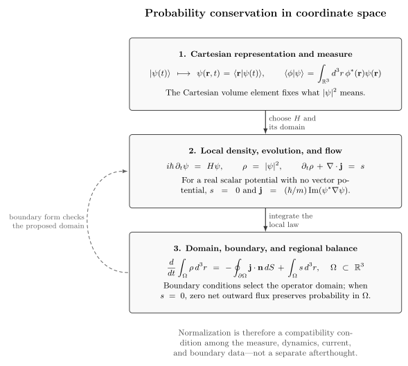
Probability conservation in coordinate space. The wavefunction determines a density and current; their local continuity equation relates the probability in a region to the flux through its boundary. A source term is needed only when the chosen effective equation supplies one.

Reading sequence

Read	Article	Capability gained
1	Coordinate Representation	Translate kets, inner products, and operators into coordinate amplitudes and kernels.
2	Wavefunctions and Probability Density	Interpret $\lvert\psi\rvert^2$ relative to the correct measure, including internal and many-particle labels.
3	Time-Dependent Schrödinger Equation in Coordinate Space	Pose a well-defined initial-value problem and distinguish the differential expression from its domain.
4	Time-Independent Schrödinger Equation	Formulate stationary spectral and boundary-value problems without treating every state as stationary.
5	Hamiltonians in Coordinate Space	Build kinetic, potential, effective, and electromagnetic differential operators with stated assumptions.
6	How to Solve a Wave-Mechanics Problem	Turn a physical setup into a domain, equation, normalized solution, and observable.
7	Probability Current	Compute direction and magnitude of probability flow, including scattering flux and gauge coupling.
8	Continuity Equation	Derive local and integral conservation and identify legitimate source or sink terms.
9	Boundary Conditions	Derive endpoint and interface conditions and connect them to self-adjointness and flux.
10	Normalization Conventions	Move correctly among square, box, delta, energy, flux, radial, and numerical normalization.
11	Expectation Values	Calculate averages with the correct operator and measure.
12	Dimensionless Variables and Scaling	Identify independent parameters and natural length and energy scales.
13	Stationary States and Expansions	Evolve a superposition using an energy basis.
14	Qualitative Features of One-Dimensional Bound States	Use nodes, parity, and asymptotic behavior before solving exactly.
15	From Wave Mechanics to Quantum Fields	After studying the relevant models, distinguish oscillator excitation from particle creation and evolution kernels from field correlators.

Use the foundations in a model

Start with representation, density, and the two Schrödinger equations. Then read boundary conditions and normalization alongside the infinite well. Current becomes especially useful for the potential step and barrier problems. Minimal coupling extends the scalar-potential equations above to electromagnetic fields.

For quick lookup after the derivation, use the current formula and continuity equation.

Exercises

1. A packet moves from left to right through an interval $[a,b]$. Relate the probability change inside the interval to the endpoint currents.

Solution

Integrating $\partial_t\rho+\partial_xj=0$ gives $dP_{[a,b]}/dt=j(a)-j(b)$. Entry at the left increases the regional probability and exit at the right decreases it. Equal currents give a stationary regional probability even though particles can flow through the interval.

2. Why does a unit-norm grid eigenvector need a scale factor before it is plotted as a continuum wavefunction?

Solution

With uniform rectangle quadrature, the continuum norm is $\sum_i|\psi(x_i)|^2\Delta x\simeq1$, whereas the array has $\sum_i|v_i|^2=1$. Thus $\psi(x_i)\simeq v_i/\sqrt{\Delta x}$. Other quadrature rules require their own weights.

References

• L. E. Ballentine, Quantum Mechanics: A Modern Development, 2nd ed., World Scientific, 2014.
• C. Cohen-Tannoudji, B. Diu, and F. Laloë, Quantum Mechanics, Wiley, 1977.
• D. J. Griffiths and D. F. Schroeter, Introduction to Quantum Mechanics, 3rd ed., Cambridge University Press, 2018.
• R. Shankar, Principles of Quantum Mechanics, 2nd ed., Springer, 1994.