Relativistic Quantum Mechanics

Relativistic quantum mechanics connects Lorentz symmetry to wave equations, spin, antiparticles and controlled approximations for matter in prescribed fields. The Klein–Gordon and Dirac equations encode relativistic dispersion; their different currents and state spaces determine what a calculation means. This volume develops those structures, applies them to electromagnetic and low-energy problems, and identifies how those results extend to quantum fields.

Begin with ordinary wave mechanics, complex linear algebra, and calculus. The Special-Relativity Toolkit teaches the Lorentz notation and conventions used here. Add electromagnetic, scattering, and Fock-space methods when the calculation needs them; the readiness checks below identify the capabilities to practise. For an ordered route from wave equations to fields, use the Bridge to QFT Roadmap.

Chapters and their purposes

Chapter	What it develops
Special-Relativity Toolkit	Conventions, Lorentz transformations, invariant measures, currents and causal geometry.
Limits of Relativistic One-Particle Quantum Mechanics	Energy sectors, localization, probability, causality and the useful range of one-particle descriptions.
Klein–Gordon	Scalar modes, conserved pairings, prescribed backgrounds and initial-value problems.
Dirac	Clifford algebra, covariant and Hamiltonian forms, normalized spinors and currents.
Spinors, Lorentz and Poincaré	Component representations, massive and massless particle states, helicity, chirality and Wigner rotations.
Electromagnetic Coupling	Gauge covariance, Dirac dynamics, FW transformations, magnetic response and atomic spectra.
Discrete Symmetries	Parity, time reversal, charge conjugation, Majorana compatibility and the CPT boundary.
Scattering and Propagators	Green kernels, normalized amplitudes, invariant phase space, unitarity and an LSZ checkpoint.
Antiparticles and Pair Creation	Charge sectors, particle-changing channels, in/out occupations and vacuum persistence.
Nonrelativistic Limits	Prepared-sector limits, Pauli/FW operators, dynamical decoupling and NRQED matching.
Bridge Concepts	Free-field constructions, correlators, generating functionals and selected QED comparisons.
Notebooks	Reproducible calculations with downloadable programs, data and analytical checks.
Reference	Convention, spinor, bilinear, normalization, propagator, Hamiltonian and symbol lookup.
Problems and Projects	Conceptual checks, derivations, numerical investigations and bounded field-theory capstones with solutions.

Kinematics, modes, and field structure

Relativistic symmetry constrains possible descriptions; it does not select a unique wave equation, state space, or interaction. A solid arrow in the figure marks a constraint, a dotted arrow marks added quantum structure, and dashed arrows mark controlled reduction or matching.

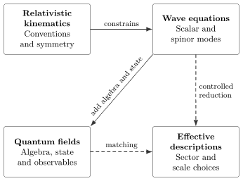
The arrows have different meanings. Symmetry alone does not select a unique wave equation; a mode equation alone does not supply a quantum algebra, interaction or observable. Effective descriptions require stated sectors and scales. TikZ source.

Input and choice	Connection and destination
Relativistic momentum and a time orientation	Constrain the mass shell and select the positive-energy invariant measure
Mass shell plus a scalar amplitude	Construct the Klein–Gordon equation
Mass shell plus a first-order Clifford/spinor construction	Construct the Dirac equation; scalar factorization relates the equations but does not make their state descriptions identical
Poincaré symmetry and a representation space	Organize spinor components or unitary particle states, with different transformation laws
Wave equations plus prescribed gauge potentials	Define external-field coupling and gauge covariance
A wave operator plus a source and boundary prescription	Define a Green-function inverse
Complex-valued modes plus oscillator algebra and a state	Construct free quantum fields and their correlations
Matter plus dynamical electromagnetic degrees of freedom and an interaction	Enter the gauge-theory and QED bridges
A retained particle sector and controlled low momenta and fields	Obtain Pauli dynamics and FW corrections

The limitations of a fixed-particle model can motivate a larger state space. They do not themselves construct its algebra, vacuum, or dynamics. See Relationship to Quantum Field Theory for the additional input needed to turn modes into a field prediction.

Preparation for each calculation

When it is needed	Capability	Where to learn it
Starting free wave mechanics	Normalize a complex state; use adjoints, observables, commutators and unitary evolution	Quantum States, Observables, Commutators and Schrödinger Equation
Reading waves and differential operators	Differentiate complex phases, use Fourier transforms, and distinguish an ODE from a PDE initial-value problem	Fourier Transform, complex/Fourier checklist and calculus/ODE/PDE checklist
Entering Dirac spinors	Multiply Pauli matrices and interpret a two-component spin state	Pauli Matrices and Spin-Half Hilbert Space
Coupling a prescribed electromagnetic field	Obtain fields from potentials; distinguish signed charge, canonical momentum and kinetic momentum	Electromagnetism checklist and minimal coupling in wave mechanics
Calculating scattering rates	Relate amplitudes, incident flux and final-state counting; use the Born approximation within its scope	First Born Approximation, Cross Sections and Relativistic Normalization
Interpreting field modes and pairs	Use occupation-number states and bosonic or fermionic creation operators	Fock Space, bosonic commutators and fermionic anticommutators

Elementary familiarity with inertial frames is useful; mastery of relativistic notation is an outcome of the toolkit, not a prerequisite for opening it. Operator domains become consequential for Hamiltonians and singular Coulomb problems; representation theory and distributions enter their corresponding chapters. Follow each article’s required background when taking an advanced branch.

Complex states. Normalize $(1,i)^{\mathsf T}$ and write its adjoint: the column is $(1,i)^{\mathsf T}/\sqrt2$ and its adjoint is the row $(1,-i)/\sqrt2$. Transposition alone is not conjugate transposition.

Plane-wave derivatives. Applying $i\hbar\partial_t$ and $-i\hbar\partial_x$ to $e^{i(px-Et)/\hbar}$ returns $E$ and $p$ times the same wave. Keep $\hbar$ explicit long enough to check dimensions.

Spin algebra. Verify $[\sigma_x,\sigma_y]=2i\sigma_z$ and explain why these two spin components cannot have a common eigenbasis.

Electromagnetic potentials. Calculate $\mathbf E=-\nabla\Phi-\partial_t\mathbf A$, $\mathbf B=\nabla\times\mathbf A$, and $\boldsymbol\pi=\mathbf p-q\mathbf A$ for a specified potential. State the charge sign before interpreting the result.

Conventions that travel with a calculation

Metric and Units fixes the mostly-minus signature, the phase $e^{-ip\cdot x/\hbar}$ and the signed charge $q$, with $q=-e$ for an electron and $e>0$. The gamma-matrix conventions fix the Clifford algebra and explicit bases. Natural units are announced where used; the Natural Units table restores dimensions and conversion factors.

Normalization and boundary prescriptions are equally consequential. Use the Normalization Table before combining external states, measures and amplitudes, and the Propagator Table before identifying a source inverse with a field correlation. These tables link to the derivations and state the conventions a formula needs.

A finite-dimensional spinor boost need not be unitary in the Euclidean component norm. A full particle state also carries its momentum measure and transformation law; Wigner classification explains the unitary particle representation.

Prescribed backgrounds and controlled reductions

Free and suitable static particle sectors can give exact subproblems; controlled one-particle approximations also remain valuable in more general settings. Low momentum, weak backgrounds, negligible recoil, and suppressed particle creation are different conditions. An exact solution of a chosen wave equation does not include every effect of its physical source.

• The Dirac Coulomb spectrum uses a specified point-nucleus model and operator realization; recoil, finite nuclear size, and radiative shifts require additional treatment.
• The Landau problem resolves levels and spin multiplicities in a uniform prescribed magnetic field. A finite matrix calculation must distinguish physical states from cutoff artifacts.
• The Klein step determines scattering flux ratios; these are not, by themselves, vacuum pair probabilities.
• The strong-field vacuum calculation adds a specified in/out field interpretation. Mean pair number and vacuum survival are different observables, and the background remains prescribed.

Low-energy descriptions also arise through different operations:

• The exact free FW transformation unitarily transforms states and observables while retaining both free energy blocks. Selecting one block is an additional restriction.
• The static FW expansion is an asymptotic calculation with specified momentum and field counting; a truncation is not an exact identity over all states.
• Antiparticle decoupling asks when dynamics approximately preserves the selected sector, within a stated norm and time regime.
• NRQED matching fixes effective coefficients by reproducing specified field-theory amplitudes or observables. It can include effects absent from a classical external-field Dirac equation.

Use When Relativistic QM Is Useful to compare omitted effects with the requested accuracy.

What changes at the field-theory boundary

A conserved Klein–Gordon charge need not be a positive local Born density; a positive Dirac density does not remove the negative-energy sector of the full one-particle Hamiltonian. The current comparison keeps those statements separate.

A quantum-field prediction specifies an operator algebra, state space, state, dynamics, and observable. Complex-valued wave-equation modes remain useful; operator coefficients supply creation and annihilation structure. The general quantum probability rules survive. Free-particle Fock space is not a universal description of every interacting or infrared state.

Relationship to Quantum Field Theory compares these structures through detector, pair-production, and scattering examples. Renormalized loops, the complete Lamb shift, dynamical non-Abelian gauge fields, and general spin–statistics or CPT proofs require a systematic field-theory treatment. Local LSZ and NRQED calculations state their narrower assumptions; charged states coupled to massless photons need qualifications beyond an isolated stable-particle pole and naive Fock asymptotic states.

Practice and further study

Pair a derivation with its topic notebook to test normalization, limiting cases and numerical convergence. The problem chapter asks you to transfer those ideas to a new calculation; its solutions separate mathematical checks from physical interpretation. The Reading List gives textbook and lecture-note assignments with convention warnings.

For compact lookup beyond the local tables, use the Relativistic QM Formula Cards and Hamiltonian Cards. Their summaries complement the detailed explanations linked throughout this volume.

References

• Bjorken, James D., and Sidney D. Drell. Relativistic Quantum Mechanics. McGraw–Hill, 1964.
• Foldy, Leslie L., and Siegfried A. Wouthuysen. “On the Dirac Theory of Spin 1/2 Particles and Its Non-Relativistic Limit.” Physical Review 78, 29–36 (1950). doi:10.1103/PhysRev.78.29.
• Greiner, Walter. Relativistic Quantum Mechanics: Wave Equations. 3rd ed., Springer, 2000. doi:10.1007/978-3-662-04275-5.
• Thaller, Bernd. The Dirac Equation. Springer, 1992. doi:10.1007/978-3-662-02753-0.
• Weinberg, Steven. The Quantum Theory of Fields, Volume I: Foundations. Cambridge University Press, 1995. doi:10.1017/CBO9781139644167.