Composite Systems and Entanglement

Two quantum systems can have a definite joint state without either subsystem having a definite pure state. Understanding that fact requires three tools: tensor products to describe the whole, partial traces to describe a part, and entanglement tests to distinguish quantum correlations from mixtures of independent preparations. This volume develops those tools through explicit two-qubit calculations before extending them to many subsystems and continuous variables.

Required background. State Vectors supplies basis expansions, and Density Operators supplies the positive trace-one operators used for mixed and reduced states. Tensor Products is a helpful linear-algebra companion.

A pair contains more information than either part

For distinguishable subsystems $A$ and $B$, the joint Hilbert space is

$$\mathcal H_{AB}=\mathcal H_A\otimes\mathcal H_B.$$

Two qubits therefore have the four basis states $|00\rangle$, $|01\rangle$, $|10\rangle$, and $|11\rangle$. Both the pure Bell state and the following classical mixture give equal probabilities for $00$ and $11$ when measured in this basis:

$$|\Phi^+\rangle=\frac{|00\rangle+|11\rangle}{\sqrt2}, \qquad \rho_{\rm mix}=\frac{|00\rangle\langle00|+|11\rangle\langle11|}{2}.$$

They are different joint states. The Bell state retains coherence between the two alternatives, whereas the mixture does not. For example, measuring $\sigma_x$ on both qubits gives

$$\langle\sigma_x\otimes\sigma_x\rangle_{\Phi^+}=1, \qquad \langle\sigma_x\otimes\sigma_x\rangle_{\rm mix}=0.$$

Yet either qubit alone has the same reduced state $I/2$ in both cases. Thus local randomness, or correlation in one basis, does not by itself establish entanglement. Classical Correlation versus Entanglement works through this comparison.

From joint states to local predictions

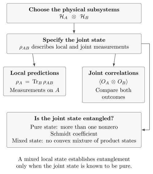
For finite-dimensional bipartite systems, a joint state answers different questions about local measurements, joint correlations, and entanglement. The subsystem split must be specified first. The entanglement test concerns the joint state; a mixed local state alone does not settle it.

Learn the calculation in stages

What you want to understand	Where to begin
Subsystem labels, product bases, and local operators	Tensor Product Foundations
Product, separable, and entangled preparations	Product, Separable, and Entangled States
Predictions for only one part of a system	Reduced States and Partial Trace
Schmidt decomposition and entanglement tests	Bipartite Entanglement
Correlations shared among three or more parts	Multipartite Entanglement
Modes, Gaussian states, and continuous variables	Continuous Variables and Modes
Connections with other areas of physics	Entanglement Across Fields
Formulas, solved problems, and computational practice	Reference, Problems, and Notebooks

For a first calculation, read Notation and Subsystem Labels, construct the tensor-product space, distinguish product and entangled states, calculate a partial trace, and then use the Schmidt decomposition. Interactions and Coupling Terms shows how a coupled pair evolves from a product state into an entangled state.

Specify the subsystems before classifying a state

Entanglement is defined relative to a specified division into subsystems and the operations available on them. A tensor factor may represent an atom, a spin register, a spatial region, or a field mode; these choices are not interchangeable.

For identical particles, formal particle labels are not individually addressable subsystems. Symmetrization and antisymmetrization alone should not be confused with operationally accessible entanglement. The Many-Body volume develops the additional structure in Identical Particles and Exchange Symmetry, Fock Space, and Second Quantization. Here the focus is the chosen subsystem structure, local predictions, and entanglement.

The distinction between a local state and a conditional state is equally important. Ignoring the outcome of a measurement on $B$ leaves $A$‘s reduced state unchanged. Conditioning on a communicated outcome can change the ensemble assigned to $A$. This explains how entangled correlations coexist with the absence of faster-than-light signalling.

Continue from structure to applications

After partial traces and Schmidt decomposition, Quantum Information explains operational tasks such as teleportation and information processing. Measurement and Open Quantum Systems develops instruments, channels, and environmental dynamics. Bell Locality and Quantum Correlations examines the assumptions tested by Bell inequalities. These applications depend on the subsystem calculations introduced here.

Exercises

Verify the two $\sigma_x\otimes\sigma_x$ expectation values above using $\sigma_x|0\rangle=|1\rangle$ and $\sigma_x|1\rangle=|0\rangle$.

Solution

The operator exchanges $|00\rangle$ and $|11\rangle$, so it leaves their equal coherent superposition $|\Phi^+\rangle$ unchanged. The Bell state is therefore an eigenstate with eigenvalue $+1$. In each product component of $\rho_{\rm mix}$ the expectation is zero: for example $\langle00|\sigma_x\otimes\sigma_x|00\rangle=\langle00|11\rangle=0$. Averaging the two components still gives zero. The difference comes from the off-diagonal terms in the Bell density operator.

References

• M. A. Nielsen and I. L. Chuang, Quantum Computation and Quantum Information, Cambridge University Press, 2010 — tensor products, reduced states, and Schmidt decomposition.
• A. Peres, Quantum Theory: Concepts and Methods, Kluwer, 1995 — composite systems and correlations.
• E. Schrödinger, “Discussion of Probability Relations between Separated Systems,” Mathematical Proceedings of the Cambridge Philosophical Society 31, 555–563, 1935 — the joint-state and subsystem distinction.
• R. Shankar, Principles of Quantum Mechanics, 2nd ed., Springer, 1994 — composite state spaces and coupled systems.