Quantum Matter Frontiers and Open Problems

Research on quantum matter connects unfamiliar signals to possible phases, excitations and mechanisms. The difficult step is often deciding which interpretation a measurement supports. A resistance anomaly, a broad spectrum and a narrow calculated band each leave several physical explanations open.

This chapter helps you turn such an observation into a question that another experiment or calculation can answer. Use the linked Library articles for the underlying physics and Quantum Matter Research for research directions, dated assessments and starter projects.

Required background. From Models to Measured Observables connects systems, states and observables.

Helpful background. How quantum matter is measured explains how detector signals become physical quantities. Data interpretation and pitfalls develops comparisons between alternative models.

From an observation to a physical explanation

Consider a neutron experiment that finds broad scattering in energy and momentum. The spectrum is a measured response. Attributing it to fractional excitations is an interpretation. Identifying a spin-liquid ground state is a further statement about the many-body phase. Explaining why a particular material realizes that phase adds a microscopic mechanism. Each step needs additional reasoning.

This distinction is useful even when a measurement is highly reproducible. Two laboratories can agree on a spectrum while disagreeing about its origin. Several analysis methods applied to the same data also share the specimen, calibration and much of the noise; agreement between those analyses is valuable but is not an independent experiment.

Ask four connected questions when reading a new result:

1. What was measured or calculated? Identify the response, operator or output, including its units and resolution. Separate measured voltages from inferred conductivity, and a finite-model eigenvalue from a thermodynamic phase.
2. For which state? Keep temperature, field, filling, geometry, disorder and preparation in view. A pulsed state can change appreciably during a probe; a surface measurement need not describe the bulk.
3. Which alternatives predict the same feature? Compare them after the same instrumental broadening and with the same definition of the observable. A poor alternative model is an easy opponent and a weak test.
4. Where do their predictions differ? Seek an accessible parameter range or complementary observable that separates the explanations by more than the combined uncertainty.

The point is to make progress even when the favored explanation remains uncertain. Showing that a proposed measurement cannot distinguish two models is a useful result: it redirects effort toward a better experiment. Keimer and Moore’s review provides a broad physical introduction to the interplay of correlations, topology and experimental probes.

Choose a physical question

The following links connect a stable explanation to a research question.

Question	Learn the physics	Explore a research direction
What pairs the electrons?	Pairing physics	Pairing research
What does linear resistivity imply?	Strange metals	Non-Fermi liquids
Are the excitations fractionalized?	Spin liquids	Spin-liquid research
What establishes non-Abelian statistics?	Braiding physics	Non-Abelian statistics
Which interacting phase forms in a Chern band?	Moiré topology	Fractional Chern insulators
How does driving change the state?	Periodic driving	Driven systems
Can a predicted property be realized?	Materials design	Materials discovery

These questions overlap, but their tests differ. Gap symmetry constrains a pairing mechanism without usually selecting it uniquely. A continuum can arise from fractionalized excitations, disorder or multiparticle processes. A local zero-bias peak is not a measurement of exchange statistics. Savary and Balents discuss the continuum ambiguity for spin liquids; Nayak and colleagues explain the fusion and braiding operations needed for non-Abelian physics.

For a proposed fractional Chern phase, compare calibrated filling and the conductivity tensor with incompressibility, temperature dependence and competing ordered states. No single universal checklist replaces a consistent explanation of the available measurements. A resistance plateau is not automatically a quantized Hall conductivity when longitudinal resistance is appreciable. Even a convincing phase identification does not directly measure fractional charge or braiding; those are separate experimental questions.

A narrow Drude peak can look inductive

A simple example shows why the measured frequency window matters. Consider a stationary linear response with time convention $e^{-i\omega t}$. A normal Drude contribution is

$$\sigma_D(\omega)=\frac{D}{\Gamma-i\omega},$$

where $D>0$ is its spectral-weight parameter and $\Gamma>0$ is an angular relaxation rate. The real part describes dissipative absorption; the imaginary part describes a current out of phase with the electric field. They are

$$\begin{aligned} \sigma_{1,D}&=\frac{D\Gamma}{\Gamma^2+\omega^2},\\ \sigma_{2,D}&=\frac{D\omega}{\Gamma^2+\omega^2}. \end{aligned}$$

At $\omega\gg\Gamma$, the imaginary part is nearly $D/\omega$. An ideal stiffness contribution has

$$\sigma_s(\omega)=\pi D_s\delta(\omega) +iD_s\,\mathcal P\frac1\omega,$$

where $\mathcal P$ denotes principal value. If $D_s=D$, their positive-frequency imaginary parts become hard to distinguish when the entire measured window lies above the Drude width.

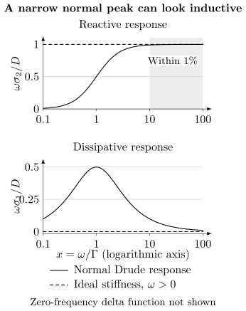
The solid curves are the exact Drude response for $x=\omega/\Gamma>0$. Dashed lines show an ideal stiffness contribution of the same weight at positive frequency; its zero-frequency delta function is not plotted. Above $x=10$, the reactive curve differs from the ideal value by less than 1%, although the Drude relaxation rate is nonzero. Lower frequencies or sufficiently precise dissipation measurements distinguish these two models.

The dimensionless combinations in the figure are

$$\begin{aligned} \frac{\omega\sigma_{2,D}}D&=\frac{x^2}{1+x^2},\\ \frac{\omega\sigma_{1,D}}D&=\frac{x}{1+x^2}. \end{aligned}$$

This is an exact counterexample to identifying phase stiffness from a finite-band $1/\omega$ trend alone. It does not show that every inductive response is a narrow Drude peak. Instead, it identifies what the experiment must resolve to separate these particular alternatives.

There is a second distinction even at ideal resolution. A clean normal conductor can have a zero-frequency Drude weight in a uniform optical response. Superconducting magnetic screening involves the transverse response and its static, long-wavelength limits, as discussed by Scalapino, White and Zhang. Optical weight and a Meissner response cannot be identified without those qualifications; London theory develops the screening response.

A short-lived state adds a time constraint

For pump–probe measurements, the state may evolve on the same timescale as the response. The measured two-time kernel need not equal an instantaneous equilibrium-like conductivity. Orenstein and Dodge demonstrate this explicitly for a photoexcited Drude model. Pump–probe spectroscopy explains how to compare models through the acquisition and detector response.

Lowering the nominal probe frequency is therefore not automatically decisive. The observation must last long enough to constrain the relevant relaxation while the evolving state is modeled consistently. Repeating a pump sequence can improve signal precision, but does not make the state in each shot live longer. A phase-sensitive or magnetic measurement must also probe the same preparation and relevant time interval.

A Planckian estimate depends on the transport model

Suppose a finite temperature window gives $\rho(T)=\rho_{\rm fit}+AT$. In a one-band Drude model with temperature-independent density $n$ and current mass $m^\star$, the transport relaxation time $\tau_{\rm tr}$ determines the resistivity through

$$\rho=\frac{m^\star}{ne^2\tau_{\rm tr}}.$$

The slope then defines

$$\begin{aligned} \alpha_{\rm tr} &=\frac{\hbar ne^2 A}{m^\star k_B},\\ \hbar\frac{d\tau_{\rm tr}^{-1}}{dT}&=\alpha_{\rm tr}k_B. \end{aligned}$$

The inference is conditional on that transport model. A Hall-derived carrier density assumes a carrier description and Hall factor; a cyclotron mass is not automatically the current mass entering a multiband conductivity. The intercept of a finite-temperature fit need not be the measured zero-temperature resistivity. A separation into residual and inelastic scattering rates requires additional additivity assumptions.

Bruin and colleagues compared rate scales in metals with linear resistivity. Hartnoll and Mackenzie explain why quasiparticle, transport and many-body relaxation times must be distinguished. An order-one value of $\alpha_{\rm tr}$ is an interesting comparison, but does not alone establish a universal bound or a microscopic mechanism. Conventional phonon scattering can also give approximately linear resistivity in appropriate regimes.

Use strange metals for the physical analysis and transport measurements for geometric and instrumental limitations. A productive next step compares several observables with one carrier and scattering model, rather than fitting each with unrelated parameters.

Make the next comparison informative

Numerical convergence answers whether a calculation reliably solves its specified approximation. It does not establish that the approximation describes the material. Compare system size, temperature, basis, interaction model and observable definition before interpreting disagreement between methods. Shared input parameters can also correlate their uncertainties.

For two scalar estimates, the uncertainty of their difference satisfies

$$\operatorname{Var}(x_1-x_2) =\sigma_1^2+\sigma_2^2 -2\operatorname{Cov}(x_1,x_2).$$

This variance is not a probability that either mechanism is correct. A small fit residual likewise does not establish a unique explanation. Test whether physically distinct models remain compatible with the data, not merely whether the favored model fits.

For experiments, separate repeat measurements, new specimens and independent laboratories. Each addresses different possible errors. Independent methods may still share density calibration, sample preparation or a theoretical conversion, so explain what has actually become independent. The National Academies’ report on reproducibility and replicability discusses these distinctions.

For a materials-discovery calculation, a ranked candidate is a proposal for further study. Test-set error averages across a population; it is not automatically the error on one unfamiliar candidate. Agreement among models trained on the same reference data can miss their shared bias. Butler and colleagues describe the broader role of machine learning in materials research. Useful follow-up work tests the predicted property under structural uncertainty and then compares it with a measurement that is sensitive to that property.

Read the date and scope of research assessments, including corrections and later tests. A result can strengthen one part of an explanation while leaving another unresolved. End a comparison with a precise statement of what the data establish and one feasible calculation or measurement that could change the interpretation.

Exercises

1. Quantify the optical ambiguity

For the stationary models above, find the relative reactive discrepancy $1-\omega\sigma_{2,D}/D$ and the ratio $\sigma_{1,D}/\sigma_{2,D}$. Evaluate both at $\omega=20\Gamma$. Does the nearly ideal reactive response prove zero relaxation?

Solution

They are $1/(1+x^2)$ and $1/x$. At $x=20$, the reactive discrepancy is $1/401\simeq0.249\%$, while the dissipative-to-reactive ratio is $5\%$. Thus a precise measurement of both components can be more discriminating than the reactive curve alone. The model has $\Gamma>0$ throughout; a nearly ideal reactive curve does not imply zero relaxation.

2. Compare the observation time with the linewidth

A trial Drude model has $\Gamma/(2\pi)=0.02\,\mathrm{THz}$, while a prepared state lasts $1.4\,\mathrm{ps}$. Estimate the relaxation time $1/\Gamma$ and the record length needed for a Fourier-bin spacing $1/T_{\rm obs}<0.02\,\mathrm{THz}$. What limitation does this expose?

Solution

The relaxation time is about $7.96\,\mathrm{ps}$. The frequency-bin criterion requires $T_{\rm obs}>50\,\mathrm{ps}$, much longer than the state lifetime. Window shape and a parametric model affect practical parameter precision, so bin spacing is not a universal resolution theorem. Nevertheless, treating this state as stationary for a long Fourier record is inconsistent. Model its time dependence and use complementary observables instead of interpreting the nominal frequency range alone.

3. Propagate a model-dependent rate estimate

Take $A=0.300\pm0.010\,\mu\Omega\,\mathrm{cm/K}$, $n=(8.0\pm1.5)\times10^{27}\,\mathrm{m}^{-3}$ and $m^\star=(5.0\pm1.0)m_e$. Use independent small-error propagation within the one-band model. Find $\alpha_{\rm tr}$ and explain what the result does not determine.

Solution

The SI slope is $3.00\times10^{-9}\,\Omega\,\mathrm{m/K}$, giving $\alpha_{\rm tr}\simeq1.033$. Its fractional standard uncertainty is

$$\begin{aligned} \left(\frac{\sigma_\alpha}{\alpha}\right)^2 &=\left(\frac{1.5}{8.0}\right)^2 +\left(\frac{1.0}{5.0}\right)^2 +\left(\frac{0.010}{0.300}\right)^2, \\ \frac{\sigma_\alpha}{\alpha}&\simeq0.276. \end{aligned}$$

Thus $\alpha_{\rm tr}=1.03\pm0.29$ under the specified model and approximation. Correlated inputs require covariance terms. Alternative carrier models add model uncertainty, which is not included in this error bar. The calculation estimates a transport-rate slope; it does not identify the single-particle lifetime, a unique scattering mechanism or a universal bound.

4. Interpret a missing magnetic Bragg peak

A neutron experiment resolves no magnetic Bragg peak down to $80\,\mathrm{mK}$ and finds a broad inelastic continuum. Its sensitivity is $0.03\mu_B$ per ion for the tested magnetic structures. Give a defensible conclusion and two complementary tests.

Solution

The experiment excludes the tested static orders above its stated sensitivity and within its momentum and time acceptance. It does not exclude all forms of order or establish a spin liquid. A local probe such as NMR or muon spin rotation can test slow freezing on a different timescale. Polarization-resolved scattering and independently characterized samples can test magnetic versus phonon contributions and the role of disorder. The choices should target explicit alternative models; a broad continuum is not unique to fractionalization.

5. Separate a boundary signal from braiding

A single tunnel contact resolves a zero-bias conductance peak in a proximitized wire. No correlated opposite-end signal, fusion protocol or exchange operation has been measured. What has been observed, and what further distinction is needed for a non-Abelian claim?

Solution

The result is a local low-energy tunneling feature. Ordinary Andreev states, confinement and disorder can produce related features, so the peak alone does not identify a topological mode. Spatial and bulk-gap information can constrain those alternatives. Even identifying candidate separated modes is distinct from demonstrating their fusion space or noncommuting exchange operations. See topological superconductors and anyons and braiding for those separate questions.

6. Test a predicted narrow band

A model predicts a bandwidth of $7\pm3\,\mathrm{meV}$, where the spread is across ten training seeds. Its held-out test RMSE is $6\,\mathrm{meV}$. Two admissible relaxation models give $9$ and $16\,\mathrm{meV}$; the desired screen is bandwidth at most $12\,\mathrm{meV}$ and separation from excluded bands at least $20\,\mathrm{meV}$. Neither calculation reports the separation. A device shows a resistance maximum. Which conclusions follow?

Solution

The seed spread measures variation among these fitted models, while RMSE summarizes test-set errors. Neither is automatically a calibrated uncertainty for this candidate. The relaxation alternatives straddle the bandwidth threshold, and the isolation condition has not been tested. A resistance maximum does not directly measure either quantity. The stated information does not verify a narrow isolated band or a correlated phase. Compute the missing separation under structural variations and choose spectroscopy or another observable that tests the predicted electronic structure.

References

• J. A. N. Bruin, H. Sakai, R. S. Perry, and A. P. Mackenzie, “Similarity of scattering rates in metals showing $T$-linear resistivity,” Science 339, 804–807 (2013). doi:10.1126/science.1227612.
• K. T. Butler, D. W. Davies, H. Cartwright, O. Isayev, and A. Walsh, “Machine learning for molecular and materials science,” Nature 559, 547–555 (2018). doi:10.1038/s41586-018-0337-2.
• S. A. Hartnoll and A. P. Mackenzie, “Colloquium: Planckian dissipation in metals,” Reviews of Modern Physics 94, 041002 (2022). arXiv:2107.07802.
• B. Keimer and J. E. Moore, “The physics of quantum materials,” Nature Physics 13, 1045–1055 (2017). doi:10.1038/nphys4302.
• National Academies of Sciences, Engineering, and Medicine, Reproducibility and Replicability in Science, National Academies Press (2019). doi:10.17226/25303.
• C. Nayak, S. H. Simon, A. Stern, M. Freedman, and S. Das Sarma, “Non-Abelian anyons and topological quantum computation,” Reviews of Modern Physics 80, 1083–1159 (2008). arXiv:0707.1889.
• J. Orenstein and J. S. Dodge, “Terahertz time-domain spectroscopy of transient metallic and superconducting states,” Physical Review B 92, 134507 (2015). arXiv:1506.06758.
• L. Savary and L. Balents, “Quantum spin liquids: A review,” Reports on Progress in Physics 80, 016502 (2017). doi:10.1088/0034-4885/80/1/016502.
• D. J. Scalapino, S. R. White, and S. Zhang, “Insulator, metal, or superconductor: The criteria,” Physical Review B 47, 7995–8007 (1993). doi:10.1103/PhysRevB.47.7995.