Gauge, Phase, and Magnetic Geometry

A magnetic field changes both the motion of a charged particle and the relative phase of its possible paths. Gauge transformations let us describe those effects using different potentials while predicting the same probabilities and currents. This chapter develops that connection between phase and electromagnetism for a nonrelativistic particle in prescribed fields. It also explains why a particle can respond to enclosed magnetic flux even when its accessible paths are field free.

Helpful background. Rays and global phase explains why an overall phase is unobservable. Minimal coupling in wave mechanics introduces the charged-particle Hamiltonian; spatial symmetries introduces translation generators.

Enter this chapter

Question	Read next
Which phases affect interference?	Global phase and local phase transformations
How must derivatives and potentials transform together?	Minimal coupling and gauge transformations
How can flux affect paths outside the field?	Aharonov–Bohm effect
Which translations survive in a uniform field?	Magnetic translations and Landau levels
What happens when one potential cannot cover the whole space?	Dirac monopole
How is magnetic phase represented on a lattice?	Peierls phase

Local phase changes require transformed potentials

For a spinless particle of signed charge $q$, use

$$H=\frac{(\mathbf p-q\mathbf A)^2}{2m}+q\Phi, \qquad \mathbf p=-i\hbar\nabla.$$

Here $\Phi$ is the electric scalar potential. The kinetic momentum $\boldsymbol\pi=\mathbf p-q\mathbf A$ gives the velocity $\mathbf v=\boldsymbol\pi/m$. The derivative in $\mathbf p$ acts on everything to its right, including a position-dependent potential when the square is expanded.

Multiplying $\psi$ by a constant phase changes no prediction. Multiplying it by $e^{iq\chi(\mathbf r,t)/\hbar}$ with the potentials held fixed generally changes the current and the physical state. A gauge change transforms the whole description:

$$\psi'=e^{iq\chi/\hbar}\psi,\qquad \mathbf A'=\mathbf A+\nabla\chi,\qquad \Phi'=\Phi-\partial_t\chi.$$

Apply the product rule once:

$$\begin{aligned} (-i\hbar\nabla-q\mathbf A')\psi' &=e^{iq\chi/\hbar} \bigl(-i\hbar\nabla+q\nabla\chi-q\mathbf A'\bigr)\psi\\ &=e^{iq\chi/\hbar}\boldsymbol\pi\psi. \end{aligned}$$

The unwanted phase gradient cancels the change in the vector potential. Thus $\boldsymbol\pi\psi$ transforms in the same way as $\psi$; this is gauge covariance. Both $|\psi|^2$ and the probability current

$$\mathbf j=\frac1m\operatorname{Re}(\psi^*\boldsymbol\pi\psi)$$

are unchanged. The time-dependent scalar-potential term is equally necessary. With $U_\chi=e^{iq\chi/\hbar}$,

$$H'=U_\chi H U_\chi^\dagger +i\hbar\dot U_\chi U_\chi^\dagger.$$

This is equivalence of Schrödinger equations, not a claim that the instantaneous Hamiltonian matrices have identical eigenvalues in every time-dependent gauge. The allowed gauge change must also transform the operator domain and boundary conditions consistently.

Local fields and closed-loop phase

The fields $\mathbf B=\nabla\times\mathbf A$ and $\mathbf E=-\nabla\Phi-\partial_t\mathbf A$ are gauge invariant. In a region with zero magnetic field, a vector potential can still have a nonzero integral around a loop that encloses excluded flux. For a static Aharonov–Bohm arrangement, the magnetic contribution to the relative phase is

$$\Delta\varphi=\frac q\hbar\oint_C\mathbf A\cdot d\mathbf r =\frac{q\Phi_B}{\hbar}\pmod{2\pi}.$$

The loop follows one path forward and the other backward; its orientation fixes the sign. Aharonov and Bohm’s analysis makes the physical distinction precise: interference measures this relative phase, not the value of the vector potential at one point.

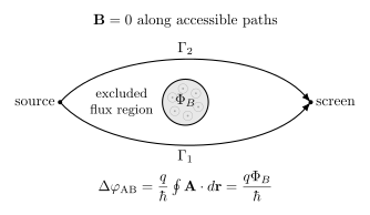
The two paths form an oriented loop around flux $\Phi_B$. The accessible paths may be field free while their magnetic relative phase is $q\Phi_B/\hbar$. Other path-dependent phases must be held fixed or accounted for in an interference comparison.

The invariant quantity is $e^{i\Delta\varphi}$. The flux period has magnitude $h/|q|$. Stokes’ theorem remains valid: a spanning disk enclosing the flux passes through the region excluded from the particle’s motion. Zero field on the accessible region does not guarantee globally removable potentials.

Translation symmetry and Landau degeneracy

Take a particle on the infinite plane, no scalar potential, and a uniform field $\mathbf B=B\hat{\mathbf z}$ with $B>0$. Then

$$[\pi_x,\pi_y]=i\hbar qB,\qquad H=\frac{\pi_x^2+\pi_y^2}{2m}.$$

This noncommuting pair produces an oscillator spectrum $E_n=\hbar\omega_c(n+1/2)$, where $\omega_c=|q|B/m$. It does not follow that $\boldsymbol\pi$ generates translations that preserve the energy: its components do not commute with $H$.

In symmetric gauge $\mathbf A=\mathbf B\times\mathbf r/2$, the conserved translation generator is instead

$$\mathbf K=\mathbf p+q\mathbf A, \qquad [K_i,\pi_j]=0, \qquad [K_x,K_y]=-i\hbar qB.$$

Consequently $T(\mathbf a)=e^{-i\mathbf a\cdot\mathbf K/\hbar}$ commutes with $H$, but translations in different directions obey

$$T(\mathbf a)T(\mathbf b) =e^{iqB(a_xb_y-a_yb_x)/\hbar} T(\mathbf b)T(\mathbf a).$$

Their order differs by the phase of the enclosed flux. A change of gauge conjugates these translation operators along with the Hamiltonian. Boundaries or a nonuniform potential may remove this translation symmetry.

The related guiding-center coordinates

$$X=x+\frac{\pi_y}{qB},\qquad Y=y-\frac{\pi_x}{qB}$$

commute with $H$ and satisfy $[X,Y]=-i\hbar/(qB)$. They describe the location of the cyclotron motion without changing its energy. This is the origin of the bulk Landau-level degeneracy, approximately $|q|B\mathcal A/h$ states per spinless level in a large area $\mathcal A$. Edge states and boundary conditions require a separate finite-system treatment.

Gauge patches and lattice links

A hypothetical monopole field $\mathbf B=g\mathbf r/r^3$ has flux $4\pi g$ through a surrounding sphere. It cannot be represented by a single smooth vector potential on the sphere. Northern and southern potentials are related on their overlap by a gauge function $\chi=2g\phi$. The transition phase $e^{i2qg\phi/\hbar}$ must be single valued, giving $2qg=n\hbar$. The monopole article derives this condition using two patches. It is a consistency condition if a monopole exists, not a prediction of its existence.

For tight-binding amplitudes $\psi_i$, a hopping matrix element from site $j$ to site $i$ instead carries a link phase

$$H_{ij}=t_{ij}e^{i\theta_{ij}},\qquad \theta_{ij}=\frac q\hbar\int_{\mathbf r_j}^{\mathbf r_i}\mathbf A\cdot d\mathbf r.$$

Changing $\psi_i\mapsto e^{iq\chi_i/\hbar}\psi_i$ changes $\theta_{ij}$ by $q(\chi_i-\chi_j)/\hbar$, preserving the lattice equation’s covariance. Endpoint phases cancel around a closed loop. The Peierls prescription is an approximation to continuum magnetic coupling; it omits changes in the localized orbitals and hopping magnitudes, and does not supply spin coupling by itself.

For a first pass, work through phase covariance and the two-path effect before the translation algebra. Then Berry geometry introduces a related connection induced by changing eigenspaces in parameter space. Gauge theory adds dynamical fields and further physical assumptions.

Exercises

1. A particle of charge $q$ travels around an excluded flux $\Phi_B$. By how much may the flux change without changing the Aharonov–Bohm interference phase?

Solution

The invariant phase is

$$W = \exp \left( \frac{iq\Phi_B}{\hbar} \right).$$

A flux change $\Delta\Phi$ leaves it unchanged when

$$\frac{q\Delta\Phi}{\hbar} = 2\pi n, \qquad n\in\mathbb Z.$$

Therefore

$$\Delta\Phi = n\frac{h}{q}.$$

In magnitude, the fundamental period is

$$\Phi_0 = \frac{h}{|q|}.$$

The sign records charge and orientation conventions; the interference depends on the phase modulo $2\pi$.

2. Derive the Dirac quantization condition from the overlap gauge function $\chi=2g\phi$.

Solution

On the overlap of the northern and southern patches,

$$\psi_N = \exp \left( \frac{i2qg\phi}{\hbar} \right) \psi_S.$$

When $\phi$ increases by $2\pi$, this transition function changes by

$$\exp \left( \frac{i4\pi qg}{\hbar} \right).$$

Single-valued patching requires the factor to equal one:

$$\frac{4\pi qg}{\hbar} = 2\pi n.$$

Hence

$$2qg=n\hbar, \qquad n\in\mathbb Z.$$

Equivalently,

$$\frac{q}{2\pi\hbar} \int_{S^2} \mathbf B\cdot d\mathbf S = n.$$

3. Show that the product of Peierls phases around a plaquette is gauge invariant.

Solution

Each oriented link phase transforms as

$$\theta_{ij}' = \theta_{ij} +\frac{q}{\hbar} \left( \chi_i-\chi_j \right).$$

Summing around a closed plaquette makes the endpoint terms telescope:

$$\sum_{\langle ij\rangle\in\partial p} \left( \chi_i-\chi_j \right) =0.$$

Therefore

$$\prod_{\langle ij\rangle\in\partial p} e^{i\theta_{ij}'} = \prod_{\langle ij\rangle\in\partial p} e^{i\theta_{ij}}.$$

For a smooth field, the common value is

$$\exp \left( \frac{iq\Phi_p}{\hbar} \right),$$

where $\Phi_p$ is the magnetic flux through the plaquette.

References

• Y. Aharonov and D. Bohm, “Significance of electromagnetic potentials in the quantum theory,” Physical Review 115, 485–491, 1959. doi:10.1103/PhysRev.115.485.
• P. A. M. Dirac, “Quantised singularities in the electromagnetic field,” Proceedings of the Royal Society A 133, 60–72, 1931.
• L. D. Landau and E. M. Lifshitz, Quantum Mechanics: Non-Relativistic Theory, 3rd ed., Pergamon, 1977.
• R. Peierls, “Zur Theorie des Diamagnetismus von Leitungselektronen,” Zeitschrift für Physik 80, 763–791, 1933.
• T. T. Wu and C. N. Yang, “Concept of nonintegrable phase factors and global formulation of gauge fields,” Physical Review D 12, 3845–3857, 1975.
• J. Zak, “Magnetic translation group,” Physical Review 134, A1602–A1606, 1964.