Geometric Phases and Topology

A slowly steered quantum state can return to its starting ray with a phase that depends on the path of the controls. This Berry phase remains after subtracting the familiar phase accumulated from energy and elapsed time. It connects interference to the geometry of eigenstates. Some global quantities built from that geometry are quantized, but an ordinary Berry phase can change continuously when the path changes.

Helpful background. Projective Hilbert space distinguishes a ray from its phase representative. Time-dependent Hamiltonians supplies the evolution equation, and differential forms explains the compact notation $A=A_i\,dR^i$ and $F=dA$ used below.

Enter this chapter

Question	Read next
Which part of a cyclic phase comes from the path?	Dynamical and geometric phase and Berry phase
When does a state follow an instantaneous eigenspace?	Adiabatic theorem reminder
How are neighboring eigenstates compared?	Berry connection and parallel transport
What do finite and infinitesimal loops measure?	Holonomy and Berry curvature
Which examples make the geometry visible?	Spin one half, Aharonov–Bohm comparison, and molecular Berry phase
When is a quantity quantized?	Chern numbers and topological quantum numbers
How does this enter band physics?	Zak phase and quantum Hall geometry
What replaces a scalar phase for degenerate states?	Non-Abelian Berry phase

Following an eigenstate around a loop

Let $H(R)|n(R)\rangle=E_n(R)|n(R)\rangle$, where $R$ denotes controls such as a magnetic-field direction. Assume a smooth, nondegenerate eigenvalue separated from the rest of the spectrum throughout a slow traversal $R(t)$, and start in that eigenstate. The standard adiabatic approximation gives

$$|\psi(t)\rangle\simeq \exp\left[-\frac i\hbar\int_0^tE_n(t')\,dt'+i\gamma_n(t)\right] |n(R(t))\rangle,$$

where $\dot\gamma_n=i\langle n|\dot n\rangle$. The approximation needs control of transitions to other levels, not merely a cyclic Hamiltonian. A useful diagnostic is

$$\frac{\hbar|\langle m|\dot H|n\rangle|}{|E_m-E_n|^2}\ll1, \qquad m\ne n.$$

This ratio identifies troublesome small gaps; by itself it is not a universal error bound for arbitrary protocols. Rigorous estimates also require appropriate smoothness, gap, and time-scaling assumptions.

For a closed parameter loop $C$, the eigenvector may return with a different phase. In any smooth gauge along the path, the geometric phase is

$$\gamma_n[C]=\int_0^T i\langle n(t)|\dot n(t)\rangle\,dt +\arg\langle n(0)|n(T)\rangle \pmod{2\pi}.$$

In a periodic gauge the endpoint term vanishes, giving $\gamma_n[C]=\oint_C A_n$. Including that endpoint comparison prevents an arbitrary choice of eigenvector phase from changing the answer. Traversing the same oriented loop more slowly leaves the geometric phase unchanged in the adiabatic limit, while generally changing the dynamical phase.

Connection, curvature, and parallel transport

The connection is the local one-form

$$A_n=i\langle n|dn\rangle.$$

It describes how the chosen eigenvector changes along infinitesimal displacements in parameter space. Rephasing $|n\rangle\mapsto e^{i\chi}|n\rangle$ gives $A_n\mapsto A_n-d\chi$. The curvature $F_n=dA_n$ is unchanged. In coordinates, $F_{ij}=\partial_iA_j-\partial_jA_i$.

A parallel-transport choice sets $i\langle n|\dot n\rangle=0$ along a path. It removes the local phase accumulation from the integral, but a parallel-transported ket can still return with an endpoint phase. That finite mismatch is called holonomy. A gauge can be parallel along the whole path or periodic around a loop with nontrivial holonomy, but cannot be both.

If one smooth gauge covers a spanning surface $\Sigma$, Stokes’ theorem gives $\oint_{\partial\Sigma}A_n=\int_\Sigma F_n$. With multiple patches, transition phases must be included. The curvature controls the phase change between nearby loops; it does not determine every holonomy on a space with noncontractible loops without further global information.

Spin one half and solid angle

Choose

$$H(\hat{\mathbf n})=-\frac\Delta2\hat{\mathbf n}\cdot\boldsymbol\sigma, \qquad \Delta>0.$$

The lower-energy state has $\hat{\mathbf n}\cdot\boldsymbol\sigma=+1$. A useful local eigenvector is

$$|+;\theta,\phi\rangle= \begin{pmatrix}\cos(\theta/2)\\e^{i\phi}\sin(\theta/2)\end{pmatrix}.$$

Direct differentiation gives

$$A_+=-\frac{1-\cos\theta}{2}\,d\phi, \qquad F_+=-\frac12\sin\theta\,d\theta\wedge d\phi.$$

Thus $\gamma_+[C]=-\Omega[C]/2$ modulo $2\pi$, where $\Omega[C]$ is the oriented solid angle enclosed by the loop. These signs refer to the Hamiltonian, eigenstate, and orientation just specified.

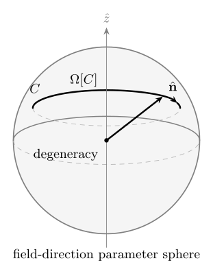
The controls trace a loop on the sphere of directions at fixed nonzero gap $\Delta$. Its solid angle determines the geometric phase. Moving the loop continuously generally changes the phase even while the energy gap remains open.

For a circle at polar angle $\theta_0$, $\gamma_+=-\pi(1-\cos\theta_0)$. A small circle around the north pole gives a small phase; the equator gives $-\pi$. An interference experiment needs a reference and a way to subtract or cancel the dynamical phase.

What topology adds

Over a closed oriented two-dimensional parameter surface $M$, an isolated smooth eigenline has an integer Chern number

$$C_n=\frac1{2\pi}\int_MF_n\in\mathbb Z.$$

For the spin example on the whole sphere, $C_+=-1$. The eigenvector written above is not smooth at the south pole; another patch is needed there. A globally smooth single eigenvector would imply a global $A_n$, and Stokes’ theorem on the closed surface would give zero total curvature flux. Nonzero $C_n$ is precisely an obstruction to that global choice.

The integer is stable under smooth deformations that preserve the isolated eigenline on all of $M$. In contrast, $\gamma[C]$ for one loop is usually continuous. A noncontractible loop alone does not quantize its phase. For a flat connection held fixed, holonomy is unchanged by a deformation within the same loop class; the value can still change when the connection changes. Additional symmetry can quantize certain phases, provided its assumptions and coordinate conventions remain fixed.

This distinction matters for the Zak phase of a one-dimensional band. Its value depends on the origin and orbital conventions, and only suitable protecting symmetries restrict it to particular values. In two dimensions, a filled, isolated collection of noninteracting bands can instead yield an integer Hall response through its total Chern number, with the sign set by charge and orientation conventions. Filling, a gap, and the response calculation are part of that physical result; topology alone is not a complete transport model.

Beyond a single isolated level

In molecular physics, electronic eigenstates depend on nuclear positions. Following one electronic surface induces a Berry connection in nuclear motion. A loop around a suitable conical intersection can produce a sign change even when real eigenvectors make the local connection vanish on each patch. Passage through the degeneracy generally requires several coupled electronic surfaces.

For an exactly degenerate eigenspace separated from other levels, a local orthonormal basis $|u_a(R)\rangle$ defines a matrix connection $A_{ab}=i\langle u_a|du_b\rangle$. After removing the common dynamical phase, adiabatic transport is

$$\mathcal U[C]=\mathcal P\exp\left(i\int_C A\right).$$

Different segments need not commute, so their order matters. In a periodic frame, changing the basis at the starting point conjugates the closed-loop matrix; its eigenvalues are unchanged. This is rotation within an isolated subspace. It does not by itself create a dynamical gauge field.

For a first pass, calculate the spin connection and the three exercises below. Then choose molecular phases, band geometry, or degenerate transport according to the physical problem you want to study.

Exercises

1. Starting from $A=i\langle n|dn\rangle$, derive the gauge transformation of the connection under $|n\rangle\mapsto e^{i\chi}|n\rangle$. Then show directly that $F=dA$ is gauge invariant.

Solution

The transformed connection is

$$\begin{aligned} A' &= i \langle n| e^{-i\chi} d \left( e^{i\chi}|n\rangle \right) \\ &= i \left( i\,d\chi + \langle n|dn\rangle \right) \\ &= A-d\chi. \end{aligned}$$

Taking an exterior derivative,

$$F' = dA' = dA-d^2\chi = F,$$

because $d^2=0$.

2. For the spin-$1/2$ convention in this page, let the field direction follow a circle of fixed polar angle $\theta_0$ with $\phi:0\to2\pi$. Find the Berry phase and its limiting values at $\theta_0=0$ and $\theta_0=\pi/2$.

Solution

The enclosed solid angle is

$$\Omega = 2\pi \left( 1-\cos\theta_0 \right).$$

Hence

$$\gamma_+ = -\frac{\Omega}{2} = -\pi \left( 1-\cos\theta_0 \right) \quad \operatorname{mod}2\pi.$$

At the north pole, $\theta_0=0$, the loop shrinks and $\gamma_+=0$. At the equator, $\theta_0=\pi/2$, the phase is $-\pi$, equivalent to $\pi$ modulo $2\pi$.

3. Integrate

$$F_+ = -\frac12 \sin\theta\,d\theta\wedge d\phi$$

over the standard oriented sphere and compute the Chern number. Which assumptions make the result meaningful?

Solution

Using $0\le\theta\le\pi$ and $0\le\phi<2\pi$,

$$\begin{aligned} \int_{S^2}F_+ &= -\frac12 \int_0^{2\pi}d\phi \int_0^\pi \sin\theta\,d\theta \\ &= -2\pi. \end{aligned}$$

Therefore

$$C_+ = \frac{1}{2\pi} \int_{S^2}F_+ = -1.$$

The sphere must be closed and oriented, and the chosen eigenstate must remain isolated at every point on the sphere. The degeneracy may lie inside the sphere, but not on it.

References

• M. V. Berry, “Quantal phase factors accompanying adiabatic changes,” Proceedings of the Royal Society A 392, 45–57, 1984. doi:10.1098/rspa.1984.0023.
• C. A. Mead and D. G. Truhlar, “On the determination of Born–Oppenheimer nuclear motion wave functions including complications due to conical intersections and identical nuclei,” Journal of Chemical Physics 70, 2284–2296, 1979.
• B. Simon, “Holonomy, the quantum adiabatic theorem, and Berry’s phase,” Physical Review Letters 51, 2167–2170, 1983.
• D. J. Thouless, M. Kohmoto, M. P. Nightingale, and M. den Nijs, “Quantized Hall conductance in a two-dimensional periodic potential,” Physical Review Letters 49, 405–408, 1982.
• D. Vanderbilt, Berry Phases in Electronic Structure Theory, Cambridge University Press, 2018.
• F. Wilczek and A. Zee, “Appearance of gauge structure in simple dynamical systems,” Physical Review Letters 52, 2111–2114, 1984.
• J. Zak, “Berry’s phase for energy bands in solids,” Physical Review Letters 62, 2747–2750, 1989.