Disorder, Localization, and Nonequilibrium Matter

Why does a wave packet stop spreading, a spin pattern retain memory, or a driven material settle into a persistent state? These observations can arise from different mechanisms. Static disorder changes the Hamiltonian from sample to sample; interactions redistribute energy within a sample; a drive supplies energy, while a reservoir can remove it. This chapter helps distinguish those effects and choose the calculation that addresses the measured behavior.

Helpful background. Tight-Binding Models supplies lattice sites, hopping and local energies. Density Operators distinguishes a quantum state from a statistical ensemble. Transport, Response, and Optics connects material observables to response functions.

Enter this chapter

Choose a starting point by the physical question. You need not study localization before investigating a periodically driven system, and a localized sample need not be glassy.

Physical question	Suggested reading
What is random?	Disorder in Quantum Matter: distributions, correlations and scattering scales
Why does coherent spreading stop?	Anderson Localization and Anderson Insulators: localized states and transport
How does interference change conductance?	Weak Localization and Scaling Theory: corrections and size dependence
What changes across the spectrum?	Mobility Edges and Random Matrix Theory: energy-resolved states and level statistics
Why does local memory persist?	Glasses and Spin Glasses and Many-Body Localization: distinct mechanisms and tests
What follows a sudden preparation?	Quenches and Quantum Thermalization: relaxation and statistical ensembles
What does a periodic drive produce?	Floquet Quantum Matter: quasienergies, occupations and heating
What do reservoirs change?	Driven-Dissipative Matter and Open Quantum Materials: steady states and reduced dynamics

Three distinctions that organize the physics

A random sample and an average over samples

In quenched disorder, the random potential is fixed during the evolution under study. Compute the observable in each fixed sample before averaging over samples. Averaging the potential first can erase the scattering that you wanted to understand. A time-fluctuating potential is a different problem: it can exchange energy and destroy phase coherence. A deterministic quasiperiodic potential is different again, even when its spatial pattern looks irregular.

Sample distributions may be broad. A few conducting samples can dominate the arithmetic mean while most samples transmit poorly. Comparing means, typical values and size dependence is therefore part of understanding transport. The scaling argument of Abrahams and colleagues (1979) organizes conductance by length; its conclusions depend on dimension, symmetry and interaction assumptions.

Weak localization is a small interference correction in a diffusive conductor. Strong localization describes a different regime, with localized eigenstates and exponentially suppressed coherent transmission over long distances. Neither a large resistance nor a fitted hopping exponent identifies the mechanism by itself. Contacts and a finite coherence length can also limit a measurement; return to the mesoscopic chapter when those scales dominate.

Stationarity, equilibration and thermalization

An observable can settle near a plateau without taking its thermal value. Thermalization additionally means agreement with the ensemble appropriate to the conserved quantities and the class of observables being tested. In an isolated system, local observables can relax while the full state evolves unitarily. Exercise 2 shows why equal mean energy alone is insufficient.

The many-body treatment of relaxation and the eigenstate thermalization hypothesis develop this connection; D’Alessio and colleagues (2016) give a pedagogical review. Integrable systems can retain extra conserved quantities. Long-lived prethermal states can resemble equilibrium before later evolution changes them.

Persistent memory also has several explanations. A glass can age: its response depends on the waiting time after preparation. A noninteracting localized system can retain memory without many-body interactions. An interacting disordered system requires comparison with those alternatives and with residual environmental coupling. The many-body localization treatment and Sierant and colleagues (2025) explain the difficulty of extrapolating finite sizes and times to asymptotic behavior. Level repulsion or Poisson-like spacing statistics alone does not resolve these distinctions.

A driven state and a state selected by a reservoir

A periodic Hamiltonian defines a one-period evolution operator, but its quasienergies do not determine which states are populated. Motion within a period also contributes to measurements. The Floquet theorem establishes the exact construction, while many-body Floquet systems explains heating and prethermal behavior.

For suitable local bounded many-body models, high-frequency driving can produce a long regime governed approximately by an effective static Hamiltonian (Abanin and colleagues, 2017). The driving frequency must be compared with the relevant local scales; many observed cycles do not by themselves justify the approximation.

With continuous pumping and loss, the state is selected by both coherent evolution and environmental processes. A stationary density operator can support continuing energy or particle fluxes and need not be a Gibbs state (Sieberer, Buchhold and Diehl, 2016). A non-Hermitian matrix may describe response poles or trajectories conditioned on no detected loss; neither interpretation alone supplies the unconditional state. Exercise 3 illustrates the difference.

For a material experiment, pump–probe spectroscopy connects preparation and detection. A changed optical signal can reflect occupations, broadening or heating as well as a changed Hamiltonian. The frontiers guide links to dated discussions of proposed phases.

When is there time to observe the intended regime?

Suppose a periodically driven sample has period $T=0.20\,\mathrm{ms}$. Over a calibrated interval of 20 ms, three measured changes are modeled by

$$\begin{aligned} a(t)&=e^{-t/\tau_r},\\ h(t)&=t/\tau_h,\\ \ell(t)&=1-e^{-t/\tau_\ell}. \end{aligned}$$

Here $a$ is the remaining preparation transient, $h$ is the energy increase divided by a declared energy scale, and $\ell$ is the lost-particle fraction. Take $\tau_r=3\,\mathrm{ms}$, $\tau_h=80\,\mathrm{ms}$ and $\tau_\ell=150\,\mathrm{ms}$. These are illustrative fitted laws, not universal relaxation or heating formulas.

At 20 ms the system has undergone 100 periods and $a\simeq0.00127$. Nevertheless, $h=0.25$ and $\ell\simeq0.125$. A small preparation transient does not guarantee that the subsequent state has remained nearly unchanged.

If all three changes must be below a tolerance $\eta$, the allowed times obey

$$\begin{aligned} t&>\tau_r\ln(1/\eta),\\ t&<\eta\tau_h,\\ t&<-\tau_\ell\ln(1-\eta). \end{aligned}$$

At $\eta=0.01$, the lower bound is 13.8 ms, while the upper bounds are 0.80 ms and 1.51 ms. No common interval exists. Measuring longer cannot fix this conflict.

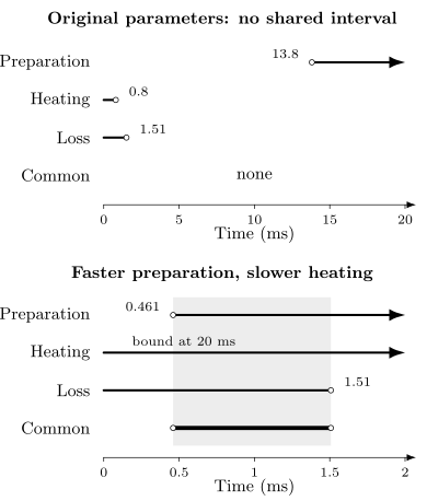
Each thick segment shows times satisfying one 1% bound. The top panel has no overlap. In the bottom panel, changing only $\tau_r$ to 0.10 ms and $\tau_h$ to 2000 ms creates a common interval from 0.461 to 1.51 ms; particle loss now sets the upper limit. The panels use different time scales. Endpoints are thresholds; the inequalities are strict.

The improved example allows several drive periods after preparation and before significant loss. This necessary timing condition still does not establish thermalization, topology or an effective Hamiltonian. The tolerances must be related to the observable: a small energy change can matter strongly near a sharp transition. Size, measurement resolution and weak-bath limits must also be examined when making long-time claims.

Exercises

1. The mean sample and the typical sample

An ensemble gives dimensionless conductance $g=1$ or $10^{-4}$ with equal probabilities and the same contact convention. Find $\langle g\rangle$ and $g_{\mathrm{typ}}=\exp\langle\ln g\rangle$. Does their difference establish localization?

Solution

The arithmetic mean is 0.50005, whereas $g_{\mathrm{typ}}=\sqrt{10^{-4}}=0.01$. The conducting half dominates the mean. This shows that a broad distribution has inequivalent summaries. A localization diagnosis still requires a specified coherent model and appropriate state or size-dependent transport tests.

2. Equal energy, different observations

Let $H=\operatorname{diag}(-\Delta,0,\Delta)$ with $\Delta>0$. Compare stationary states $\rho_A=\operatorname{diag}(1/2,0,1/2)$ and $\rho_B=\operatorname{diag}(0,1,0)$. Find their mean energies and the probabilities of the middle level. What does an energy match leave undetermined?

Solution

Both mean energies are zero, but the middle-level probabilities are zero and one. Both states commute with $H$, so stationarity does not remove the difference. Equal mean energy therefore does not identify the state or all its observables. This finite-system example does not contradict ETH, which concerns specified many-body Hamiltonians, energy windows and observables.

3. Conditioning on no detected decay

A two-level system starts in $(|g\rangle+|e\rangle)/\sqrt2$. Its only evolution is amplitude damping with $L=\sqrt\gamma\,|g\rangle\langle e|$. For ideal monitoring, compare the excited population conditioned on no detected jump with the population in the full ensemble when $e^{-\gamma t}=1/2$. Find the probability of the no-jump outcome.

Solution

The unnormalized no-jump state is

$$|\widetilde\psi_0(t)\rangle =\frac{|g\rangle+e^{-\gamma t/2}|e\rangle}{\sqrt2}.$$

Its squared norm is $3/4$, the probability of no jump. Normalizing gives excited population $(1/2)/(1+1/2)=1/3$. The full ensemble instead has excited population $e^{-\gamma t}/2=1/4$. Jumped trajectories are in the ground state, so weighting the no-jump answer gives $(3/4)(1/3)=1/4$ as required.

Lindblad operators supply the unconditional evolution. With inefficient monitoring, “no detected jump” can include an undetected decay and is no longer the pure conditional state used here.

References

• D. A. Abanin, W. De Roeck, W. W. Ho, and F. Huveneers, “Effective Hamiltonians, prethermalization, and slow energy absorption in periodically driven many-body systems,” Physical Review B 95, 014112 (2017), doi:10.1103/PhysRevB.95.014112. Controlled effective dynamics and their finite validity interval.
• E. Abrahams, P. W. Anderson, D. C. Licciardello, and T. V. Ramakrishnan, “Scaling Theory of Localization: Absence of Quantum Diffusion in Two Dimensions,” Physical Review Letters 42, 673–676 (1979), doi:10.1103/PhysRevLett.42.673. Foundational conductance-scaling argument with model-dependent scope.
• L. D’Alessio, Y. Kafri, A. Polkovnikov, and M. Rigol, “From quantum chaos and eigenstate thermalization to statistical mechanics and thermodynamics,” Advances in Physics 65, 239–362 (2016), doi:10.1080/00018732.2016.1198134. Connects spectral structure, observable matrix elements and thermalization.
• L. M. Sieberer, M. Buchhold, and S. Diehl, “Keldysh field theory for driven open quantum systems,” Reports on Progress in Physics 79, 096001 (2016), doi:10.1088/0034-4885/79/9/096001. Drive, dissipation and collective nonequilibrium descriptions.
• P. Sierant, M. Lewenstein, A. Scardicchio, L. Vidmar, and J. Zakrzewski, “Many-body localization in the age of classical computing,” Reports on Progress in Physics 88, 026502 (2025), doi:10.1088/1361-6633/ad9756. Finite-size and finite-time diagnostics and their extrapolation limits.