Many-Body Localization Preview

Many-body localization, or MBL, is a proposed regime of interacting, isolated, strongly disordered quantum matter in which local observables retain memory, transport is suppressed, and highly excited eigenstates fail the eigenstate thermalization hypothesis. Its distinctive phenomenology combines localization with interaction-induced dephasing: particles or spins can remain locally constrained even while entanglement spreads slowly across increasing distances.

That concise definition needs an unusually careful status label. Finite chains and finite-time experiments display a robust collection of MBL-like signatures. Quasilocal-integral, or l-bit, models explain those signatures coherently. A rigorous construction exists for a restricted one-dimensional random spin chain under an additional level-statistics assumption. Yet the existence and boundary of a generic asymptotic MBL phase, especially in higher dimensions or near a putative transition, remain active questions because rare resonances and thermal avalanches can occur on scales far beyond exact diagonalization and current experiments.

Finite-time memory, a useful l-bit model, and a stable infinite-system phase are different claims. This article develops the models and calculations behind those distinctions. For dated assessments and open questions, see Many-body localization research.

Helpful background. Thermalization explains the local thermal comparison, ETH describes thermal eigenstates, and entanglement entropy supplies the subsystem measure used below.

Localization, interactions, and slow relaxation

Anderson localization

Anderson localization is a single-particle interference phenomenon. For a noninteracting lattice Hamiltonian with sufficiently localized one-particle orbitals $\phi_\alpha(i)$,

$$|\phi_\alpha(i)| \lesssim C_\alpha e^{-|i-i_\alpha|/\xi_\alpha},$$

the mode occupations

$$n_\alpha = d_\alpha^\dagger d_\alpha$$

are conserved. A many-fermion Slater determinant then retains memory because each occupied localized orbital remains occupied. Entanglement created from a product state typically spreads only over one-particle localization lengths and saturates rapidly.

Many-body localization

MBL asks whether localization-like memory can survive interactions at finite energy density. Interactions invalidate independent one-particle occupations, but in a fully localized effective description they dress those occupations into quasilocal conserved pseudospins. Interactions then produce configuration-dependent phases and dephasing without efficient transport.

Slow thermalization

A thermal system can relax extremely slowly. Griffiths regions, approximate conservation laws, bottlenecks, kinetic constraints, small diffusion constants, and prethermal plateaus can all imitate localization over a finite window. A decaying observable is not localized merely because the fitted exponent is small.

Integrability

Clean integrable systems fail ordinary Gibbs thermalization because an extensive structured charge hierarchy survives. MBL phenomenology instead relies on spatially quasilocal memory tied to disorder. Both can show Poisson-like level statistics and ETH failure, so neither diagnostic identifies the mechanism alone.

Fragmentation and scars

Hilbert-space fragmentation disconnects sectors through constraints. Quantum scars concern atypical states within an otherwise thermal spectrum. A fully MBL claim concerns typical states in a declared finite-energy-density window, not a small exceptional subspace.

Regime	Interactions	Spatial disorder required	Local memory	Typical entanglement feature
Anderson insulator	no	commonly yes	yes	rapid saturation after a product-state quench
MBL-like regime	yes	random or quasiperiodic in canonical examples	yes over the tested window	slow, often logarithmic growth
clean integrable system	yes or no	no	charge-dependent	quasiparticle- and ensemble-dependent
prethermal regime	yes	no requirement	temporary	growth followed by eventual thermalization
fragmented system	yes	no requirement	sector-dependent	controlled by accessible component
thermal chaotic system	yes	no requirement	no generic local plateau	typically rapid growth toward a thermal value

Benchmark Random-Field Spin Chain

A standard numerical test bed is the spin-$1/2$ XXZ chain with a longitudinal random field,

$$H ={} J\sum_{i=1}^{L-1} \left( S_i^xS_{i+1}^x + S_i^yS_{i+1}^y \right) + J\Delta \sum_{i=1}^{L-1} S_i^zS_{i+1}^z + \sum_{i=1}^{L} h_iS_i^z.$$

For a common random ensemble,

$$h_i \overset{\mathrm{iid}}{\sim} \operatorname{Unif}[-W,W].$$

Use dimensionless spin operators $S_i^\alpha=\sigma_i^\alpha/2$, so $J$ and $h_i$ have energy units. Below, set $\hbar=k_B=1$ and measure distances in lattice spacings. Restoring units replaces $Jt$ by $Jt/\hbar$.

To compare two calculations, also specify:

• open or periodic boundaries;
• the anisotropy $\Delta$ and energy unit $J$;
• the conserved total magnetization sector;
• the distribution of $h_i$ and whether its width is $W$ or $2W$;
• the target energy density;
• the number of disorder realizations;
• whether observables are averaged arithmetically, geometrically, or through their full distribution.

The Hamiltonian conserves

$$S_{\mathrm{tot}}^z = \sum_iS_i^z.$$

Every spectral statistic must therefore be computed inside a fixed magnetization sector. Additional exact spatial symmetries must also be resolved when they survive a special disorder realization or boundary choice.

Fermion representation

Under the Jordan–Wigner transformation, write

$$S_i^z = n_i-\frac12.$$

For open boundaries, the model becomes

$$H ={} \frac{J}{2} \sum_{i=1}^{L-1} \left( c_i^\dagger c_{i+1} + c_{i+1}^\dagger c_i \right) + J\Delta \sum_{i=1}^{L-1} \left(n_i-\frac12\right) \left(n_{i+1}-\frac12\right) + \sum_{i=1}^{L} h_i \left(n_i-\frac12\right).$$

At $\Delta=0$, this is a noninteracting one-dimensional disordered hopping problem. Its localized one-particle orbitals give an Anderson insulator. At $\Delta\neq0$, the density–density term couples occupations and supplies the interaction needed for MBL phenomenology.

This comparison is unusually valuable because it changes one structural ingredient while preserving disorder:

$$\begin{gathered} \Delta=0: \\ \text{localized modes}, \\ \text{no interaction dephasing}, \\[4pt] \Delta\neq0: \\ \text{localized memory}, \\ \text{interaction-induced dephasing}. \end{gathered}$$

The clean uniform XXZ chain is Bethe-ansatz integrable. Generic random fields break translation invariance and that conventional clean-chain integrability. Calling the random-field model “integrable” merely because a finite matrix has spectral projectors would erase the locality criterion that matters.

Operational Meaning of Localization

A finite spin chain has a discrete spectrum and recurrent unitary dynamics; a generic observable need not have a pointwise long-time limit. MBL diagnostics are therefore statements about local probes, scaling, and ordered limits.

Let $O_i$ be a local Hermitian operator. A connected memory correlator in a stationary state $\rho_0$ can be written

$$C_i(t) ={} \operatorname{Tr} \left[ \rho_0 O_i(t)O_i \right] - \operatorname{Tr}(\rho_0O_i(t)) \operatorname{Tr}(\rho_0O_i).$$

The normalized identity in a chosen symmetry sector is a convenient stationary state. Subtract trivial projections onto ordinary global conserved quantities when they would otherwise supply a finite-size plateau. This connected correlator is not a universal test for every preparation: an initial eigenstate of $O_i$ can have zero connected variance while retaining its initial expectation perfectly.

A localization claim seeks a nonvanishing local component after taking the thermodynamic limit. A time-averaged version, which does not assume pointwise relaxation, is

$$\lim_{T\to\infty}\frac1T\int_0^Tdt\, \lim_{L\to\infty}C_i(t) \neq 0,$$

with the thermodynamic limit taken first for bulk dynamics. A finite-$L$ time average can still be useful, but it is not the same object.

For subsystem thermalization, compare

$$\rho_A(t) = \operatorname{Tr}_{\bar A}\rho(t)$$

with the thermal reduced state selected by the conserved densities. MBL-like behavior means that local late-time data depend on more information about $\rho_0$ than energy, particle number, and ordinary global symmetries retain.

Fully localized and energy-window claims

A fully many-body-localized model is intended to have localized structure throughout its many-body spectrum, apart from explicitly excluded sectors or exceptional states. An energy-window claim is weaker: it concerns a declared range of energy density.

This distinction matters because a thermal band elsewhere in the spectrum can act as a source of resonances. Proposed many-body mobility edges therefore require more scrutiny than a finite-size plot separating two spectral regions.

Quasilocal Integrals of Motion

The l-bit description is the central phenomenological language of a fully localized regime. Suppose a quasilocal unitary $U$ dresses physical spins into conserved pseudospins,

$$\tau_i^z = U(2S_i^z)U^\dagger, \qquad [H,\tau_i^z]=0.$$

This definition uses Pauli normalization throughout the l-bit formulas:

$$(\tau_i^z)^2 = \mathbb I.$$

Quasilocality means that the operator has exponentially decreasing tails away from site $i$. For an expansion over operators $X$ with support reaching distance $r$,

$$\|\tau_{i,r}^z\| \lesssim C e^{-r/\xi_{\mathrm{op}}}.$$

It does not mean that $\tau_i^z$ acts on one site exactly.

Effective diagonal Hamiltonian

If the $\tau_i^z$ form a complete commuting set, the Hamiltonian can be expanded as

$$H_{\mathrm{lbit}} ={} E_0 + \sum_i\widetilde h_i\tau_i^z + \sum_{i<j}J_{ij}\tau_i^z\tau_j^z + \sum_{i<j<k} J_{ijk} \tau_i^z\tau_j^z\tau_k^z + \cdots.$$

Typical effective couplings decrease with their support diameter. A schematic estimate is

$$|J_{i_1\cdots i_m}| \sim J_0 \exp \left[ -\frac{ \operatorname{diam}(i_1,\ldots,i_m) }{\xi_{\mathrm{int}}} \right].$$

A useful locality assumption must also control the sum over the many terms of a given diameter; decay of each coefficient alone is insufficient when their number grows rapidly. Under the complete l-bit description, every eigenstate is labeled by a string

$$\tau_i^z|{\boldsymbol\tau}\rangle = \tau_i|{\boldsymbol\tau}\rangle, \qquad \tau_i=\pm1.$$

The effective Hamiltonian contains no $\tau_i^x$ or $\tau_i^y$ terms, so the pseudospin populations do not flip. The interaction terms nevertheless make each pseudospin’s precession frequency depend on distant pseudospin configurations. That produces dephasing and entanglement without ordinary transport.

What the l-bit picture does not guarantee

The expansion is not a theorem for every strongly disordered Hamiltonian. Its limitations include:

• resonant clusters where perturbative dressing is not local;
• nonuniqueness under quasilocal redefinitions of conserved operators;
• possible breakdown near a transition;
• rare thermal inclusions that invalidate a global complete set;
• sensitivity to long-range interactions and unbounded local Hilbert spaces;
• exact destruction by generic coupling to an external bath.

Spectral projectors $|n\rangle\langle n|$ always commute with a finite Hamiltonian. They are highly nonlocal and do not count as l-bits.

Why ETH Fails in the Localized Description

A physical local operator overlaps with nearby l-bits. Schematically,

$$O_i = a_i\tau_i^z + \sum_j a_{ij}\tau_i^z\tau_j^z + O_i^{\perp},$$

where the coefficients decrease with distance and $O_i^{\perp}$ contains terms off diagonal in the l-bit basis.

The diagonal expectation value in an eigenstate depends on nearby labels,

$$\langle{\boldsymbol\tau}|O_i|{\boldsymbol\tau}\rangle \approx a_i\tau_i + \sum_j a_{ij}\tau_i\tau_j + \cdots.$$

Two adjacent-energy eigenstates need not share those local labels. Their local expectations can therefore remain different as $L$ grows, contrary to diagonal ETH smoothness.

After a quench, the diagonal ensemble retains the initial weights of many l-bit configurations. An energy-only Gibbs state discards that spatially resolved memory. This is not the same as the generalized Gibbs ensemble of a clean Bethe-integrable model: the conserved objects, spatial structure, disorder ensemble, and stability questions differ.

Eigenstate Diagnostics

Excited-state entanglement

In a fully localized l-bit picture, a quasilocal unitary maps product pseudospin eigenstates to physical eigenstates. Across a cut, only dressing terms near the boundary contribute appreciably, suggesting an excited-state area law in one dimension,

$$S_A(|n\rangle) = O(1)$$

for a fixed cut and typical localized eigenstates.

A thermal finite-energy-density eigenstate instead has

$$S_A(|n\rangle) \simeq s_{\mathrm{th}}(e)|A|$$

when $A$ is smaller than its complement and ETH assumptions hold. Area-law eigenstates are strong evidence, but integrable, constrained, or specially constructed states can also be low entangled.

Adjacent-gap ratio

Let sorted levels within one irreducible symmetry sector have gaps

$$\delta_n = E_{n+1}-E_n.$$

Define

$$r_n = \frac{ \min(\delta_n,\delta_{n+1}) }{ \max(\delta_n,\delta_{n+1}) }.$$

For an uncorrelated Poisson spectrum,

$$\langle r\rangle_{\mathrm P} = 2\ln2-1 \approx 0.3863.$$

For the Gaussian orthogonal ensemble,

$$\langle r\rangle_{\mathrm{GOE}} \approx 0.5307.$$

The GOE benchmark applies only when the antiunitary symmetry class and sector choice match it. Poisson-like statistics are compatible with localization, but also with integrability, unresolved block structure, or accidental degeneracy. Many-Body Quantum Chaos Preview explains symmetry classes, spectral correlations, and the Thouless scale.

Local matrix elements

Useful ETH-breaking tests include:

• broad eigenstate-to-eigenstate fluctuations of local diagonal elements;
• off-diagonal elements inconsistent with ETH entropy scaling;
• nonthermal reduced density matrices;
• persistent overlap between local operators and conserved quasilocal components.

No one small-system statistic establishes an asymptotic phase.

Quench Diagnostics

Quenches make local memory directly observable. Prepare a simple product state, evolve under the disordered interacting Hamiltonian, and record several independent channels.

Density imbalance

For a charge-density-wave preparation, let $N_{\mathrm e}(t)$ and $N_{\mathrm o}(t)$ be populations on initially occupied and initially empty sublattices. The imbalance is

$$\mathcal I(t) = \frac{ N_{\mathrm e}(t)-N_{\mathrm o}(t) }{ N_{\mathrm e}(t)+N_{\mathrm o}(t) }.$$

When the thermal state has equal mean populations on the two sublattices, thermalization predicts

$$\mathcal I(t) \longrightarrow 0$$

in the appropriate ordered limits. For an inhomogeneous sample at finite temperature, compare instead with its thermal imbalance $\mathcal I_{\mathrm{th}}$, which need not vanish. A plateau in $\mathcal I-\mathcal I_{\mathrm{th}}$ signals excess memory over the observed window. It does not by itself distinguish an asymptotic MBL phase from Anderson localization, a prethermal plateau, kinetic constraints, or very slow thermalization.

Local autocorrelation

In the fixed zero-total-magnetization sector, a common infinite-temperature spin diagnostic is

$$C(t) = \frac{1}{L} \sum_i \frac{ \operatorname{Tr} \left[ S_i^z(t)S_i^z \right] }{ \operatorname{Tr}\mathbb I }.$$

Here both traces are restricted to that sector. With $S^z=\sigma_z/2$, $C(0)=1/4$; multiply by four if a unit-normalized curve is desired. Thermal diffusion, subdiffusion, localization, and finite-size saturation produce different long-time structures. Fits must vary the lower time cutoff, system size, boundary conditions, and disorder ensemble.

Transport and number fluctuations

Localization should constrain more than one pattern. Examine:

• spreading of a domain wall or density packet;
• mean-square displacement;
• particle-number fluctuations across a cut;
• dc and low-frequency conductivity;
• response to boundary reservoirs;
• energy transport when energy is the relevant conserved density.

Slow particle transport and slow entanglement are logically distinct. An interaction can transmit phase information without carrying a conserved particle across the same distance.

Logarithmic Entanglement Growth

The clearest conceptual distinction between Anderson and MBL-like dynamics is interaction-induced dephasing.

Assume effective two-l-bit couplings decay as

$$J_{ij} \sim J_0e^{-|i-j|/\xi_{\mathrm{int}}}.$$

Two l-bits a distance $r$ apart accumulate an order-one relative phase when

$$tJ_0e^{-r/\xi_{\mathrm{int}}} \sim 1.$$

Solving for the dephasing distance gives

$$r(t) \sim \xi_{\mathrm{int}} \ln(J_0t).$$

If the initial state has nonzero diagonal entropy density $s_{\mathrm{diag}}$ in the l-bit basis, the entangled region near a cut grows with this distance:

$$S_A(t) \sim s_{\mathrm{diag}} \xi_{\mathrm{int}} \ln(J_0t)$$

over the l-bit regime before finite-size saturation.

This argument explains a hierarchy:

$$\begin{aligned} \text{Anderson:}\quad & S_A(t)\text{ saturates quickly}, \\ \text{MBL-like:}\quad & S_A(t)\propto\ln t, \\ \text{thermal:}\quad & S_A(t)\text{ grows rapidly}. \end{aligned}$$

The coefficient is not universal. Higher-body couplings, initial-state structure, rare resonances, interaction range, Rényi index, and proximity to a crossover all matter.

Extensive saturation is not thermalization

For a finite bipartition, logarithmic growth can eventually reach an extensive value,

$$S_A^{\mathrm{sat}} \propto |A|.$$

The saturation value refers to a late-time scale or average, not exact convergence of a finite system. Its coefficient can remain below the thermal entropy density and depend on the initial state. A volume-law late-time state therefore does not by itself prove ETH or transport.

Logarithmic light cone

Inverting the dephasing relation gives

$$t(r) \sim J_0^{-1} e^{r/\xi_{\mathrm{int}}}.$$

This exponentially large time for distant influence is often called a logarithmic light cone. It is much slower than a ballistic front, but it still represents unbounded spreading in an ideal infinite l-bit model.

Comparing localization signatures

Observable	Thermal expectation	MBL-like expectation	Main confound
excess imbalance $\mathcal I(t)-\mathcal I_{\mathrm{th}}$	decays to zero	nonzero long-time memory	slow crossover or Anderson localization
local autocorrelation	decays	persistent component	finite-size plateau
adjacent-gap ratio	random-matrix value	Poisson-like value	integrability or mixed sectors
eigenstate entropy	thermal volume law	area law in fully localized regime	atypical states or small sizes
quench entropy	rapid growth	slow, often logarithmic growth	broad preasymptotic window
particle transport	finite transport coefficient or hydrodynamic spreading	absent in ideal localized regime	tiny coefficient below resolution
local ETH fluctuations	shrink with size	remain broad	insufficient disorder samples
local response to perturbation	spreads and thermalizes	quasilocal memory	approximate conservation

A persuasive analysis uses several rows and tests whether one parameter regime explains them consistently.

Disorder Averages and Typicality

Quenched disorder makes observables random variables over samples. The arithmetic mean

$$\overline X = \frac1{N_s} \sum_{\alpha=1}^{N_s} X_\alpha$$

can be dominated by rare realizations. For positive $X$, a typical value is often represented by

$$X_{\mathrm{typ}} = \exp \left[ \frac1{N_s} \sum_{\alpha=1}^{N_s} \ln X_\alpha \right].$$

Neither summary replaces the distribution. Near a putative transition, report:

• median and quantiles;
• sample-to-sample variance;
• the number and selection of realizations;
• whether samples are paired across system sizes;
• bootstrap or other uncertainty intervals;
• sensitivity to rare-event trimming;
• arithmetic and typical behavior when physically meaningful.

A long-tailed distribution is physics, not merely inconvenient noise.

Random and quasiperiodic potentials

Random disorder contains arbitrarily atypical regions in the infinite system. A quasiperiodic field such as

$$h_i = W \cos(2\pi\beta i+\phi), \qquad \beta\notin\mathbb Q,$$

is deterministic for fixed phase $\phi$ and lacks the same random rare-region statistics. It can still localize and exhibit long-lived interacting nonergodicity, but its transition and stability need not share the random problem’s universality.

Calling a quasiperiodic potential “random disorder” hides precisely the distinction that avalanche and Griffiths arguments use.

Resonances

Localization perturbation theory fails when two configurations $|a\rangle$ and $|b\rangle$ satisfy

$$|\langle a|V|b\rangle| \gtrsim |E_a-E_b|.$$

An isolated resonance can be diagonalized as a larger local block. The harder question is whether resonances remain sparse and localized or connect into structures that thermalize an unbounded region.

The many-body density of states grows exponentially with volume. Consequently, a region can have an exponentially small level spacing even when every microscopic coupling is modest.

Thermal Avalanches

Consider an internally thermal inclusion of length $\ell$ with entropy density $s$. Its many-body level spacing scales schematically as

$$\delta_{\mathrm{bath}}(\ell) \sim \Lambda e^{-s\ell},$$

where $\Lambda$ is a microscopic bandwidth scale. Its coupling to a localized degree of freedom a distance $r$ away may scale as

$$g(r) \sim g_0e^{-r/\xi}.$$

The distinction between a coupling coefficient and an individual many-body matrix element matters. If the thermal region has $D\sim e^{s\ell}$ accessible states and its bounded local coupling operator obeys ETH, a typical matrix element has scale

$$v(r,\ell)\sim \frac{g(r)}{\sqrt D}, \qquad \frac{v}{\delta_{\mathrm{bath}}} \sim \frac{g(r)}{\Lambda}e^{s\ell/2}.$$

This estimate suppresses frequency-dependent spectral factors and polynomial bandwidth corrections. It assumes the bath has available transitions at the neighbor’s energy cost. If $v$ exceeds the relevant spacing, the neighbor can hybridize. Absorbing it enlarges the bath and decreases its level spacing; further absorption may then become easier. That feedback is a thermal avalanche, provided the decreasing couplings do not halt it.

What the argument establishes

Avalanche reasoning provides a stringent consistency test:

• a rare thermal region cannot be treated as a passive defect;
• stability depends on localization length, entropy density, dimension, and matrix-element scaling;
• an apparently localized finite chain may lie below an enormous avalanche length;
• thermal and localized regions must be coupled self-consistently.

What it does not establish automatically

The schematic inequalities do not supply one universal critical disorder. Matrix elements, spectral functions, conserved quantities, geometry, correlations in the disorder, and back reaction all matter. Numerical toy baths can test the mechanism without proving that a rare seed occurs with the required probability in the original model.

Dimensional caution

In higher dimensions, the boundary of a growing thermal inclusion expands and avalanche constraints become more severe. Generic fully MBL phases with random short-range disorder in $d>1$ are therefore not established and are widely viewed as unstable under plausible assumptions.

One-dimensional systems remain subtler. Restricted rigorous constructions and l-bit phenomenology support localization in particular settings, while large finite-size drifts and avalanche scales make generic extrapolation difficult. The conclusion depends on the Hamiltonian and the assumptions of the construction. The research discussion compares changing numerical extrapolations and stability arguments.

Mobility Edges Require Extra Caution

A many-body mobility edge would separate localized and thermal eigenstates by energy density. Suppose a finite spectrum appears to contain both. Then a localized region of the spectrum may couple through many-body resonances to thermal states or thermal spatial inclusions.

Before claiming an edge, test:

1. whether the apparent crossing drifts with $L$;
2. whether energy-window widths shrink consistently;
3. whether the thermal region can seed an avalanche;
4. whether the disorder ensemble admits rare inclusions;
5. whether the diagnostic agrees across spectra, eigenstates, and dynamics;
6. whether a long-lived crossover explains the same data.

An energy-resolved finite-size crossover is a valid observation. Calling it an asymptotic mobility edge is the additional claim.

Finite-size and finite-time scaling

Exact diagonalization commonly reaches only a few dozen spin-$1/2$ sites, while the Hilbert-space dimension in a half-filled sector is

$$\dim\mathcal H_{S^z=0} = \binom{L}{L/2} \sim \frac{2^L}{\sqrt{\pi L/2}}.$$

This exponential growth creates a dangerous mismatch: the hypothesized crossover or avalanche length may exceed every simulated $L$.

Crossing plots

For a dimensionless diagnostic $R(W,L)$, one may try

$$\begin{gathered} x = (W-W_c)L^{1/\nu}, \\ R(W,L) = F(x) + L^{-\omega}G(x). \end{gathered}$$

A stable inference requires more than a visually pleasing crossing:

• omit successively smaller sizes and track parameter drift;
• vary the fitting interval and polynomial order;
• include irrelevant corrections only when the data constrain them;
• propagate disorder-sampling uncertainty;
• compare random and quasiperiodic ensembles separately;
• check whether the extracted exponent respects applicable disorder bounds;
• report covariance and goodness of fit.

If $W_c$ moves systematically as the minimum size increases, the drift is part of the result.

Time-window fits

Suppose an imbalance is fit to

$$\mathcal I(t) \sim t^{-\beta}.$$

A tiny $\beta$ does not prove a plateau. Repeat the fit while moving both endpoints, compare power-law, logarithmic, stretched-exponential, and plateau-plus-decay models, and inspect residuals. If the inferred asymptote changes with the window, only a crossover has been measured.

Boundary and conservation effects

Open boundaries can thermalize or localize differently from the bulk on accessible sizes. A conserved $U(1)$ charge introduces hydrodynamic structure on the thermal side. Long-range interactions can connect distant resonances. Each feature belongs in the scaling variables, not in a footnote.

Restricted Rigorous Results

Imbrie’s one-dimensional spin-chain construction is a landmark because it builds a sequence of local rotations that diagonalizes a strongly disordered interacting Hamiltonian and controls resonant regions. The proof assumes a bound on level attraction and applies to a particular class of random chains.

It establishes neither:

• a theorem for every random-field Heisenberg or XXZ chain;
• the numerical location of a transition in the benchmark model;
• stability in arbitrary dimensions;
• stability under arbitrary long-range interactions;
• exact localization after coupling to an environment.

The correct lesson is positive but bounded: many-body localization is mathematically realizable in an interacting one-dimensional setting under explicit assumptions.

Coupling to an Environment

Exact MBL is an isolated-system concept. Let

$$H_{\mathrm{tot}} = H_{\mathrm S} + H_{\mathrm B} + gH_{\mathrm{SB}}.$$

For a generic bath with a continuum of available frequencies, $g\neq0$ gives l-bits finite transition rates. Even weak coupling can eventually erase local memory:

$$\tau_{\mathrm{bath}} \sim \Gamma^{-1}, \qquad \Gamma \propto g^2 \mathcal S_{\mathrm B}(\omega)$$

in a weak-coupling golden-rule regime.

An experiment can still display a broad intrinsic MBL-like window when

$$\tau_{\mathrm{micro}} \ll t_{\mathrm{obs}} \ll \tau_{\mathrm{bath}}.$$

This is valuable nonequilibrium physics, but the environmental lifetime must be measured rather than silently sent to infinity. Open Quantum Systems develops the reduced-dynamics framework, and Decoherence Timescales compares the relevant decay times.

What experiments measure

Quantum simulators can prepare low-entanglement states, tune disorder and interactions, and measure site-resolved observables. Their strongest contribution is direct access to dynamical mechanisms.

Quasiperiodic fermions

The 2015 optical-lattice experiment by Schreiber and collaborators observed persistent charge-density-wave imbalance in interacting fermions subject to a quasiperiodic potential. Comparing interacting and noninteracting evolution helped separate simple Anderson memory from interaction-dependent dynamics.

The measured plateau established nonergodic behavior over the available sizes and times. The experiment did not by itself take the thermodynamic and infinite-time limits.

Two-dimensional and long-range platforms

Experiments have reported slow relaxation and memory in two-dimensional optical lattices and programmable trapped-ion chains with power-law interactions. These platforms widen the phenomenology, but they also change the stability problem: dimension and interaction range are not harmless implementation details.

Entanglement measurements

Interference of identical copies and randomized measurements have enabled access to Rényi entropies and correlations. Observing continued slow entanglement growth while particle transport remains suppressed supports the interacting-dephasing picture more strongly than imbalance alone.

Engineered thermal inclusions

The 2023 cold-atom avalanche experiment coupled a tunable thermal inclusion to a localized region and observed site-resolved spreading of thermalization. This probes the avalanche mechanism directly. It is evidence about how a prepared seed acts, not by itself a measurement of the probability of spontaneous rare seeds in an infinite disorder ensemble.

Interpreting an experimental time window

Report:

• the microscopic Hamiltonian and calibration uncertainty;
• random versus quasiperiodic potential;
• preparation fidelity and initial-state energy distribution;
• system size and boundary inhomogeneity;
• observation window in tunneling times;
• interaction, disorder, and bath timescales;
• atom loss, heating, and dephasing controls;
• disorder or phase averaging protocol;
• more than one memory, transport, or entanglement observable.

Variants and Boundaries

Quasiperiodic localization

Quasiperiodic systems remove conventional random rare regions but introduce phase, commensurability, and finite-approximant effects. They deserve their own scaling analysis rather than being pooled with random chains.

Long-range interactions

If couplings decay algebraically,

$$J(r) \sim \frac{J_0}{r^\alpha},$$

distant resonances are parametrically stronger than in a short-range l-bit model. Stability depends on $\alpha$, dimension, conservation laws, and whether interactions or hopping carry the long-range tail.

Stark and disorder-free localization

Strong gradients, kinetic constraints, gauge sectors, and fragmentation can produce long-lived nonergodic dynamics without quenched disorder. These mechanisms may imitate selected MBL diagnostics but do not inherit the full random l-bit argument automatically.

Driven systems

Periodic driving removes ordinary energy conservation and can lead to heating, prethermal behavior, or proposed Floquet-localized regimes. See Floquet systems for that distinction. A driven problem requires Floquet eigenstates and an analysis of drive-induced resonances.

Worked Microexamples

Two interacting l-bits

Consider

$$H = h_1\tau_1^z + h_2\tau_2^z + J_{12}\tau_1^z\tau_2^z.$$

Prepare each pseudospin in a superposition of its $\tau^z$ eigenstates. The conditional precession frequency of pseudospin 1 is

$$\omega_1(\tau_2) = 2h_1 + 2J_{12}\tau_2.$$

Because the phase of pseudospin 1 depends on $\tau_2$, the initially factorized state becomes entangled on a timescale

$$t_{\mathrm{ent}} \sim |J_{12}|^{-1}.$$

Neither $\tau_1^z$ nor $\tau_2^z$ changes. For the initial state $|+x,+x\rangle$, tracing out spin 2 gives eigenvalues

$$\lambda_\pm(t)=\frac{1\pm|\cos(2J_{12}t)|}{2}.$$

The one-spin entropy is $h_2(\lambda_+)$, where $h_2(p)=-p\ln p-(1-p)\ln(1-p)$. It reaches $\ln2$ at $|J_{12}|t=\pi/4$ and returns to zero at $|J_{12}|t=\pi/2$. Both $\tau^z$ populations remain $1/2$ throughout. The local fields change phases by local rotations and leave this entropy unchanged. Two spins show recurrent entanglement; a broad hierarchy of weak couplings is needed for the many-spin logarithmic growth estimate.

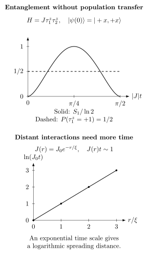
For two initially transverse l-bits, the interaction changes relative phases and hence the reduced-state entropy, while each $\tau^z$ population stays at $1/2$. The lower panel illustrates $J(r)=J_0e^{-r/\xi}$: a phase of order one appears at $J_0t\sim e^{r/\xi}$. This hierarchy motivates a logarithmic spreading distance; the two-spin recurrence alone is not a many-body localization test.

Local memory from conserved overlap

Decompose a local operator using the Hilbert–Schmidt inner product at infinite temperature,

$$O_i = a_i\tau_i^z + O_i^\perp, \qquad \operatorname{Tr} \left( \tau_i^zO_i^\perp \right) = 0.$$

The conserved component remains:

$$\tau_i^z(t) = \tau_i^z.$$

Normalize the inner product by the Hilbert-space dimension $D$ and take $O_i$ and $\tau_i^z$ traceless. Conservation and orthogonality make the cross terms vanish at every time:

$$\frac{\operatorname{Tr}[O_i(t)O_i]}D =|a_i|^2+ \frac{\operatorname{Tr}[O_i^\perp(t)O_i^\perp]}D.$$

The long-time average of the second term is a sum of nonnegative squared matrix elements inside equal-energy blocks. Thus the time-averaged autocorrelation is at least $|a_i|^2$. This is a conserved-overlap bound; it does not require the remainder to vanish or a pointwise limit to exist.

Exercises

Exercise 1: Identify the interaction

Map the random-field XXZ chain to spinless fermions and identify which term disappears at the Anderson limit.

Solution

Jordan–Wigner gives

$$S_i^z = n_i-\frac12$$

and turns the transverse exchange into nearest-neighbor hopping. The Hamiltonian is

$$H ={} \frac J2 \sum_i \left( c_i^\dagger c_{i+1} + \mathrm{h.c.} \right) + J\Delta \sum_i \left(n_i-\frac12\right) \left(n_{i+1}-\frac12\right) + \sum_i h_i \left(n_i-\frac12\right).$$

The $J\Delta$ density–density term is the interaction. At $\Delta=0$, the problem is quadratic and its one-particle eigenmodes can Anderson-localize.

Exercise 2: Derive the Poisson gap-ratio mean

For independent exponential gaps $x,y$ with unit mean, show that

$$r = \frac{\min(x,y)}{\max(x,y)}$$

has mean $2\ln2-1$.

Solution

By symmetry, integrate over $0<x<y$ and double:

$$\langle r\rangle = 2 \int_0^\infty dy \int_0^y dx\, e^{-x-y} \frac{x}{y}.$$

Set $x=uy$, with $0<u<1$ and $dx=y\,du$:

$$\langle r\rangle = 2 \int_0^1du\,u \int_0^\infty dy\, y e^{-(1+u)y}.$$

Since

$$\int_0^\infty y e^{-ay}\,dy = \frac1{a^2},$$

we obtain

$$\langle r\rangle = 2 \int_0^1 \frac{u}{(1+u)^2}\,du = 2\ln2-1.$$

Exercise 3: Recover logarithmic dephasing

Suppose $J(r)=J_0e^{-r/\xi}$. Find the largest separation that can acquire an order-one interaction phase by time $t$.

Solution

The phase scale is

$$\varphi(r,t) \sim tJ_0e^{-r/\xi}.$$

Setting $\varphi\sim1$ gives

$$r(t) \sim \xi\ln(J_0t).$$

If each newly dephased layer contributes a roughly constant entropy density across a one-dimensional cut, then

$$S_A(t) \propto \xi\ln(J_0t).$$

The derivation assumes exponentially decaying effective interactions and a suitable initial superposition in the l-bit basis.

Exercise 4: Separate transport from entanglement

Explain how the two-l-bit Hamiltonian can generate entanglement while every l-bit population remains fixed.

Solution

Because

$$[H,\tau_i^z]=0,$$

the probabilities for $\tau_i^z=\pm1$ do not change. The interaction

$$J_{12}\tau_1^z\tau_2^z$$

nevertheless assigns different phases to the four joint configurations. Starting from a product of transverse superpositions, those configuration-dependent phases prevent the state from remaining factorizable. Entanglement grows through conditional dephasing, not through transfer of the conserved $\tau^z$ populations.

Exercise 5: Diagnose an apparent plateau

A chain of sizes $L=12,14,16,18$ shows an imbalance close to $0.2$ at the latest measured time, but the late-time decay exponent decreases from $0.12$ to $0.04$ when the fitting window is moved later. What can be concluded?

Solution

The data establish long-lived memory over the simulated window. They do not establish a nonzero asymptotic plateau. The changing exponent shows that the chosen power law is not stable under the choice of time window.

Useful next tests are:

• extend time and size independently;
• compare plateau-plus-decay, logarithmic, power-law, and stretched-exponential models;
• inspect sample-level distributions;
• test transport and entanglement in the same regime;
• compare boundary conditions;
• estimate whether the accessible sizes lie below a proposed avalanche or crossover length.

Exercise 6: Thermal-bubble threshold

A thermal inclusion has $D=e^{s\ell}$ accessible states, spacing $\delta=\Lambda/D$, and a bare coupling coefficient $g_0<\Lambda$ to its neighbor. Assume a typical local bath matrix element is $D^{-1/2}$ and the required frequency is available. Estimate the seed length for first-neighbor hybridization.

Solution

The many-body coupling matrix element is $v=g_0e^{-s\ell/2}$. The comparison $v\gtrsim\delta$ gives

$$\frac{g_0}{\Lambda}e^{s\ell/2}\gtrsim1, \qquad \ell\gtrsim\frac2s\ln\frac{\Lambda}{g_0}.$$

Comparing the bare coefficient $g_0$ directly with $\delta$ misses a factor of two in this exponential estimate. If a symbol $g$ instead already denotes an individual many-body matrix element, $g\gtrsim\delta$ is appropriate, but its bath-size dependence must still be included. Continued avalanche growth also requires updating the coupling, bath spectrum, conserved sectors, and geometry at every step.

Exercise 7: Random versus quasiperiodic

Why can two potentials with comparable one-site histograms have different localization crossovers?

Solution

A one-site histogram does not encode spatial correlations. Independent random fields produce arbitrarily rare low-disorder or high-disorder regions in an infinite sample. A quasiperiodic potential has deterministic long-range correlations and does not generate the same probability distribution of rare thermal inclusions.

Consequently, Griffiths dynamics, avalanche seeding, finite-size drift, and critical scaling can differ even when the marginal distribution of field values looks similar.

Exercise 8: Design an experimental claim

An optical-lattice experiment observes nonzero imbalance for $100$ tunneling times. List the additional observations and controls needed before calling this an observation of an asymptotic MBL phase.

Solution

At minimum, establish:

• scaling across available system sizes and observation times;
• stability of the apparent plateau under later fitting windows;
• an interaction-dependent distinction from the noninteracting Anderson limit;
• a second channel such as entanglement, number fluctuations, or packet spreading;
• controls for heating, loss, dephasing, and trap inhomogeneity;
• the random or quasiperiodic character of the potential;
• sample or phase distributions rather than only an average;
• consistency with thermal-inclusion and rare-region tests.

Even then, the experimentally precise claim is finite-time, finite-size MBL-like dynamics unless the asymptotic limits are independently controlled.

Related physical questions

• Anderson localization develops the noninteracting baseline; Anderson insulators explains bath-assisted hopping in solids.
• Mobility edges distinguishes single-particle spectral coexistence from an interacting many-body edge.
• Glasses and spin glasses treats slow, history-dependent kinetics, which need not imply localized eigenstates.
• Many-body localization across platforms compares experimental observables and limitations; current research treats unresolved asymptotic stability.

References

• D. A. Abanin, E. Altman, I. Bloch, and M. Serbyn, “Colloquium: Many-Body Localization, Thermalization, and Entanglement,” Reviews of Modern Physics 91, 021001 (2019). doi:10.1103/RevModPhys.91.021001
• P. W. Anderson, “Absence of Diffusion in Certain Random Lattices,” Physical Review 109, 1492–1505 (1958). doi:10.1103/PhysRev.109.1492
• J. H. Bardarson, F. Pollmann, and J. E. Moore, “Unbounded Growth of Entanglement in Models of Many-Body Localization,” Physical Review Letters 109, 017202 (2012). doi:10.1103/PhysRevLett.109.017202
• D. M. Basko, I. L. Aleiner, and B. L. Altshuler, “Metal–Insulator Transition in a Weakly Interacting Many-Electron System with Localized Single-Particle States,” Annals of Physics 321, 1126–1205 (2006). doi:10.1016/j.aop.2005.11.014
• B. Bauer and C. Nayak, “Area Laws in a Many-Body Localized State and Its Implications for Topological Order,” Journal of Statistical Mechanics: Theory and Experiment 2013, P09005 (2013). doi:10.1088/1742-5468/2013/09/P09005
• J.-y. Choi, S. Hild, J. Zeiher, P. Schauß, A. Rubio-Abadal, T. Yefsah, V. Khemani, D. A. Huse, I. Bloch, and C. Gross, “Exploring the Many-Body Localization Transition in Two Dimensions,” Science 352, 1547–1552 (2016). doi:10.1126/science.aaf8834
• W. De Roeck and F. Huveneers, “Stability and Instability towards Delocalization in Many-Body Localization Systems,” Physical Review B 95, 155129 (2017). doi:10.1103/PhysRevB.95.155129
• L. Fleishman and P. W. Anderson, “Interactions and the Anderson Transition,” Physical Review B 21, 2366–2377 (1980). doi:10.1103/PhysRevB.21.2366
• S. Gopalakrishnan, M. Müller, V. Khemani, M. Knap, E. Demler, and D. A. Huse, “Low-Frequency Conductivity in Many-Body Localized Systems,” Physical Review B 92, 104202 (2015). doi:10.1103/PhysRevB.92.104202
• I. V. Gornyi, A. D. Mirlin, and D. G. Polyakov, “Interacting Electrons in Disordered Wires: Anderson Localization and Low-$T$ Transport,” Physical Review Letters 95, 206603 (2005). doi:10.1103/PhysRevLett.95.206603
• D. A. Huse, R. Nandkishore, and V. Oganesyan, “Phenomenology of Fully Many-Body-Localized Systems,” Physical Review B 90, 174202 (2014). doi:10.1103/PhysRevB.90.174202
• J. Z. Imbrie, “On Many-Body Localization for Quantum Spin Chains,” Journal of Statistical Physics 163, 998–1048 (2016). doi:10.1007/s10955-016-1508-x
• J. Léonard, S. Kim, M. Rispoli, A. Lukin, R. Schittko, J. Kwan, E. Demler, D. Sels, and M. Greiner, “Probing the Onset of Quantum Avalanches in a Many-Body Localized System,” Nature Physics 19, 481–485 (2023). doi:10.1038/s41567-022-01887-3
• D. J. Luitz, N. Laflorencie, and F. Alet, “Many-Body Localization Edge in the Random-Field Heisenberg Chain,” Physical Review B 91, 081103(R) (2015). doi:10.1103/PhysRevB.91.081103
• D. J. Luitz, F. Huveneers, and W. De Roeck, “How a Small Quantum Bath Can Thermalize Long Localized Chains,” Physical Review Letters 119, 150602 (2017). doi:10.1103/PhysRevLett.119.150602
• A. Lukin, M. Rispoli, R. Schittko, M. E. Tai, A. M. Kaufman, S. Choi, V. Khemani, J. Léonard, and M. Greiner, “Probing Entanglement in a Many-Body-Localized System,” Science 364, 256–260 (2019). doi:10.1126/science.aau0818
• A. Morningstar, L. Colmenarez, V. Khemani, D. J. Luitz, and D. A. Huse, “Avalanches and Many-Body Resonances in Many-Body Localized Systems,” Physical Review B 105, 174205 (2022). doi:10.1103/PhysRevB.105.174205
• V. Oganesyan and D. A. Huse, “Localization of Interacting Fermions at High Temperature,” Physical Review B 75, 155111 (2007). doi:10.1103/PhysRevB.75.155111
• A. Pal and D. A. Huse, “Many-Body Localization Phase Transition,” Physical Review B 82, 174411 (2010). doi:10.1103/PhysRevB.82.174411
• A. C. Potter, R. Vasseur, and S. A. Parameswaran, “Universal Properties of Many-Body Delocalization Transitions,” Physical Review X 5, 031033 (2015). doi:10.1103/PhysRevX.5.031033
• V. Ros, M. Müller, and A. Scardicchio, “Integrals of Motion in the Many-Body Localized Phase,” Nuclear Physics B 891, 420–465 (2015). doi:10.1016/j.nuclphysb.2014.12.014
• A. Rubio-Abadal, J.-y. Choi, J. Zeiher, S. Hollerith, J. Rui, I. Bloch, and C. Gross, “Many-Body Delocalization in the Presence of a Quantum Bath,” Physical Review X 9, 041014 (2019). doi:10.1103/PhysRevX.9.041014
• M. Schreiber, S. S. Hodgman, P. Bordia, H. P. Lüschen, M. H. Fischer, R. Vosk, E. Altman, U. Schneider, and I. Bloch, “Observation of Many-Body Localization of Interacting Fermions in a Quasirandom Optical Lattice,” Science 349, 842–845 (2015). doi:10.1126/science.aaa7432
• M. Serbyn, Z. Papić, and D. A. Abanin, “Universal Slow Growth of Entanglement in Interacting Strongly Disordered Systems,” Physical Review Letters 110, 260601 (2013). doi:10.1103/PhysRevLett.110.260601
• M. Serbyn, Z. Papić, and D. A. Abanin, “Local Conservation Laws and the Structure of the Many-Body Localized States,” Physical Review Letters 111, 127201 (2013). doi:10.1103/PhysRevLett.111.127201
• P. Sierant and J. Zakrzewski, “Challenges to Observation of Many-Body Localization,” Physical Review B 105, 224203 (2022). doi:10.1103/PhysRevB.105.224203
• P. Sierant, M. Lewenstein, A. Scardicchio, L. Vidmar, and J. Zakrzewski, “Many-Body Localization in the Age of Classical Computing,” Reports on Progress in Physics 88, 026502 (2025). doi:10.1088/1361-6633/ad9756
• J. Smith, A. Lee, P. Richerme, B. Neyenhuis, P. W. Hess, P. Hauke, M. Heyl, D. A. Huse, and C. Monroe, “Many-Body Localization in a Quantum Simulator with Programmable Random Disorder,” Nature Physics 12, 907–911 (2016). doi:10.1038/nphys3783
• T. Szołdra, P. Sierant, M. Lewenstein, and J. Zakrzewski, “Catching Thermal Avalanches in the Disordered XXZ Model,” Physical Review B 109, 134202 (2024). doi:10.1103/PhysRevB.109.134202
• T. Thiery, F. Huveneers, M. Müller, and W. De Roeck, “Many-Body Delocalization as a Quantum Avalanche,” Physical Review Letters 121, 140601 (2018). doi:10.1103/PhysRevLett.121.140601