Decoherence Timescales

A decoherence timescale is a time extracted from the decay of an interference signal, an off-diagonal density-matrix element, a pointer-state overlap, or a visibility envelope. It is not a universal property of a device or object by itself. It is a property of a model, a basis or pair of alternatives, a protocol, an environment, and a threshold convention.

An exponential envelope, a Gaussian Ramsey envelope, and a spin-echo signal can have different decay times in the same device. A useful estimate names the signal, pulse sequence, and threshold rather than reporting one universal number.

Helpful background. Dephasing vs Dissipation distinguishes population relaxation from phase decay. Environment-Induced Decoherence derives rates from environmental interactions.

Coherence envelopes and threshold times

Choose the coherence whose loss matters. For a two-level system in a chosen basis,

$$\rho = \begin{pmatrix} \rho_{00}&\rho_{01}\\ \rho_{10}&\rho_{11} \end{pmatrix},$$

the relevant coherence may be $\rho_{01}$. For energy spacing $E_1-E_0=\hbar\omega_0>0$, a simple exponential model writes

$$\rho_{01}(t) = e^{i\omega_0t} e^{-t/T_2} \rho_{01}(0).$$

Then $T_2$ is the time at which the magnitude of this off-diagonal term has fallen by $e^{-1}$:

$$|\rho_{01}(T_2)| = e^{-1} |\rho_{01}(0)|.$$

For a position superposition, the relevant object might instead be an off-diagonal position-space element:

$$\rho(x,x';t).$$

For a matter-wave interferometer, it may be fringe visibility. For a detector pointer, it may be the overlap of environmental record states. The first step in estimating a timescale is therefore not plugging numbers into a formula; it is identifying the coherence or visibility whose decay is physically relevant.

Timescale Vocabulary

The same experiment can involve several distinct times.

Symbol	Meaning	Typical diagnostic
$T_1$	population relaxation time	energy populations approach equilibrium
$T_2$	transverse coherence decay time	off-diagonal energy-basis coherence decays
$T_\phi$	pure-dephasing time	extra phase decay after separating $T_1$
$T_2^*$	inhomogeneous Ramsey decay time	ensemble or slow-noise dephasing without echo
$T_{2,\mathrm{echo}}$	echo coherence time	decay after a spin-echo pulse
$t_{\mathrm{dec}}(\Delta x)$	spatial decoherence time	position coherence at separation $\Delta x$ decays

These are fitted or inferred quantities, not microscopic mechanisms by themselves. Saying “the decoherence time is $10\,\mu\mathrm{s}$” is incomplete unless the basis, protocol, and envelope are specified.

Markovian Qubit Estimate

For a weakly coupled qubit with energy relaxation and independent pure dephasing, a constant-rate relaxation-plus-dephasing generator gives

$$\frac{1}{T_2} = \frac{1}{2T_1} + \frac{1}{T_\phi}.$$

This relation is one of the most useful quick estimates in spectroscopy and quantum-device work. It says:

• population relaxation reduces coherence at half the population-relaxation rate;
• pure dephasing adds directly to transverse coherence decay;
• $T_2$ cannot exceed $2T_1$ in this simple model unless the assumptions or fitted definitions differ.

Equivalently, with relaxation rate $\Gamma_1=1/T_1$ and pure-dephasing rate $\Gamma_\phi=1/T_\phi$,

$$\Gamma_2 = \frac{\Gamma_1}{2} + \Gamma_\phi, \qquad T_2=\Gamma_2^{-1}.$$

The precise model is a fixed-basis qubit generator with jump terms $\Gamma_\downarrow\mathcal D[|0\rangle\langle1|]+\Gamma_\uparrow\mathcal D[|1\rangle\langle0|]+(\Gamma_\phi/2)\mathcal D[Z]$, with constant nonnegative rates. Weak coupling and suitable bath approximations are one microscopic route to this generator. Nonexponential decay, leakage, driving, or changing noise conditions can make fitted time constants incompatible with it. For the generator-level derivations, see Pure Dephasing Master Equation and Amplitude Damping Master Equation.

Deriving the Half-Rate Rule

At zero temperature, amplitude damping gives

$$\dot\rho_{11} = -\Gamma_1\rho_{11}, \qquad \dot\rho_{01} = -\frac{\Gamma_1}{2}\rho_{01}$$

in the interaction picture. The excited population decays as

$$\rho_{11}(t) = e^{-\Gamma_1t}\rho_{11}(0),$$

while coherence involving the excited state decays as

$$\rho_{01}(t) = e^{-\Gamma_1t/2}\rho_{01}(0).$$

Pure dephasing with rate $\Gamma_\phi$ contributes

$$\rho_{01}(t) \longmapsto e^{-\Gamma_\phi t}\rho_{01}(t)$$

without changing $\rho_{00}$ or $\rho_{11}$. Multiplying the two independent coherence factors gives

$$\rho_{01}(t) = e^{-(\Gamma_1/2+\Gamma_\phi)t} \rho_{01}(0),$$

so

$$\frac{1}{T_2} = \frac{\Gamma_1}{2} + \Gamma_\phi.$$

The half-rate is easy to forget because populations and amplitudes decay differently. A finite-time amplitude-damping channel makes the same point: the population survival factor is $e^{-t/T_1}$, while the coherence factor is its square root, $e^{-t/(2T_1)}$.

Finite-Temperature Relaxation

At finite temperature, upward and downward transition rates both contribute to $T_1$:

$$\frac{1}{T_1} = \Gamma_\uparrow+\Gamma_\downarrow.$$

The transverse decay rate in the same simple Markovian model is

$$\frac{1}{T_2} = \frac{\Gamma_\uparrow+\Gamma_\downarrow}{2} + \Gamma_\phi.$$

Thermal excitation, spontaneous emission, engineered reservoirs, and leakage can all change what should be included in the measured relaxation rate. Before using the formula, identify the modeled subspace and decide whether leakage outside it is part of $T_1$, a separate loss channel, or a failure of the two-level description.

Ramsey, Echo, and T2*

Many experiments report a Ramsey decay time $T_2^*$ rather than the Markovian free-induction $T_2$. The star often signals inhomogeneous dephasing: slow detuning noise, static disorder across an ensemble, calibration drift, or shot-to-shot variation.

For a qubit with stochastic detuning $\xi(t)$,

$$H(t) = -\frac{\hbar}{2} [\omega_0+\xi(t)]\sigma_z,$$

with $Z=\operatorname{diag}(1,-1)$, define the rotating-frame Ramsey factor using $\rho_{10}$ (the conjugate of $\rho_{01}$):

$$W(T) = \left\langle e^{-i\int_0^T\xi(t)\,dt} \right\rangle.$$

If $\xi$ is quasi-static during each run and Gaussian distributed between runs with variance $\sigma^2$, then

$$W(T) = e^{-\sigma^2T^2/2}.$$

This is a Gaussian envelope, not an exponential Markovian one. The threshold time defined by $|W(T_*)|=e^{-1}$ is

$$T_*=\frac{\sqrt2}{\sigma}.$$

A spin echo can refocus static or slow components by reversing the sign of phase accumulation halfway through the sequence. This distinction is especially important for One-Over-F Noise, where the spectrum is concentrated near low frequencies. Echo therefore often gives a longer time than Ramsey:

$$T_{2,\mathrm{echo}} \gt T_2^*$$

when low-frequency noise dominates. Dynamical decoupling extends this logic by using pulse sequences to filter different noise bands. For filter functions and executable examples, see Dynamical Decoupling and Decoherence Timescale Estimation.

Noise-Spectrum Estimate

For centered, stationary classical Gaussian frequency noise and ideal sign-reversing control pulses, write

$$W(T)=e^{-\chi(T)}.$$

With modulation function $y(t)$ and

$$Y(\omega,T) = \int_0^T y(t)e^{i\omega t}\,dt,$$

define $C(\tau)=\langle\xi(t+\tau)\xi(t)\rangle$ and the two-sided angular-frequency spectrum

$$S_{\xi\xi}(\omega)=\int_{-\infty}^{\infty}d\tau\,e^{i\omega\tau}C(\tau).$$

The Gaussian phase average gives

$$\chi(T) = \frac12 \int_{-\infty}^{\infty} \frac{d\omega}{2\pi}\, S_{\xi\xi}(\omega) |Y(\omega,T)|^2.$$

The coherence time may then be defined by the threshold

$$\chi(T_*)=1.$$

For quasi-static noise, $S(\omega)=2\pi\sigma^2\delta(\omega)$, so only $Y(0,T)=\int y(t)dt$ matters. Ramsey has $Y(0,T)=T$; an ideal symmetric echo has $Y(0,T)=0$ and cancels this contribution exactly.

For ideal white frequency noise with $S(\omega)=S_0$, Parseval’s identity instead gives $\chi(T)=S_0T/2$ for any $y(t)=\pm1$. Echo does not remove this Markovian contribution. Real pulses add errors and real spectra have finite bandwidth, so echo need not improve every measured signal.

The formula uses angular frequency and a two-sided spectrum. With $\xi$ in radians per second, $S$ has units of inverse seconds and $\chi$ is dimensionless. Translate one-sided spectra and ordinary frequencies before substituting numbers.

For the bath side of this language, see Noise Spectra.

Spatial Decoherence

For spatial superpositions, a common reduced description is

$$\rho(x,x';t) \approx e^{-F(x-x')t} \rho(x,x';0),$$

where $F(\Delta x)$ is a separation-dependent decoherence rate. For small separations compared with the relevant environmental wavelength, one often obtains

$$F(\Delta x) \simeq \Lambda|\Delta x|^2.$$

The $e^{-1}$ time for coherence between two positions separated by $\Delta x$ is then

$$t_{\mathrm{dec}}(\Delta x) = \frac{1}{\Lambda|\Delta x|^2}.$$

The quadratic scaling means that doubling the separation reduces the decoherence time by a factor of four in this regime. For larger separations, a single scattering event may resolve the alternatives, and $F(\Delta x)$ can saturate near the scattering rate. The correct interpolation depends on wavelengths, cross sections, scatterer density, velocity distribution, geometry, and what information the environment retains.

This is the central lesson of environment-induced spatial decoherence: macroscopic separation can make environmental records highly distinguishable, so position coherence can disappear much faster than energy relaxation or mechanical damping.

A numerical Ramsey and echo comparison

Let $T_1=10\,\mu\mathrm{s}$ and let a static detuning vary independently between runs with standard deviation $\sigma=0.1\,\mu\mathrm{s}^{-1}$. Assume ideal pulses and independent Markovian relaxation. The normalized Ramsey envelope is

$$|W_R(T)|=\exp\!\left[-\frac{T}{2T_1}-\frac{\sigma^2T^2}{2}\right].$$

At $T=10\,\mu\mathrm{s}$, the two exponent contributions are each $1/2$, giving $|W_R|=e^{-1}$. The ideal echo cancels static detuning but not relaxation:

$$|W_E(T)|=e^{-T/(2T_1)}.$$

Its $e^{-1}$ time is $20\,\mu\mathrm{s}$. The two measured times differ without any contradiction, and the echo still respects the relaxation limit of this model.

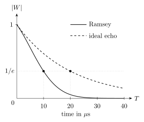
The same qubit has a $10\,\mu\mathrm{s}$ Ramsey threshold and a $20\,\mu\mathrm{s}$ ideal-echo threshold. Echo refocuses quasi-static detuning; both signals retain the same relaxation factor. Pulse imperfections and faster noise are omitted.

For independent Poisson scattering events, the corresponding rate is instead $R(1-\operatorname{Re}\eta)$, exactly within that model. Its reciprocal is an $e^{-1}$ time only when the rate is positive. Environment-Induced Decoherence derives this result and spatial-resolution limits.

Comparing Timescales

A useful hierarchy is:

$$t_{\mathrm{gate}}, \quad t_{\mathrm{meas}}, \quad t_{\mathrm{dec}}, \quad T_1, \quad t_{\mathrm{thermal}}, \quad t_{\mathrm{rec}}.$$

Here $t_{\mathrm{gate}}$ may be a control or interaction time, $t_{\mathrm{meas}}$ a measurement duration, $t_{\mathrm{dec}}$ a coherence-loss time for selected alternatives, $T_1$ an energy-relaxation time, $t_{\mathrm{thermal}}$ a thermalization time, and $t_{\mathrm{rec}}$ a recurrence or recoherence time. Their ordering depends on the system.

Examples:

• In a good qubit, gates must be much shorter than the relevant coherence envelope.
• In a measurement apparatus, pointer decoherence should be much faster than record readout.
• In macroscopic spatial decoherence, $t_{\mathrm{dec}}$ can be far shorter than mechanical damping.
• In quantum sensing, the optimal interrogation time can be close to a protocol-specific coherence time but also depends on readout, duty cycle, and signal waveform.

The phrase “decoheres before it relaxes” usually means $T_2\ll T_1$ or $t_{\mathrm{dec}}\ll T_1$. It does not mean that energy exchange is impossible, only that the interference signal vanishes on a shorter timescale than population relaxation.

Reporting a decay time

Report the observable or visibility, the basis or separation, the pulse sequence, and the fitted envelope. State whether the number is an $e^{-1}$ threshold or a parameter from a fit over a specified interval. If there are revivals, identify the first threshold crossing or the time window; there may be no unique decay constant.

For a reproducible calculation that compares these choices, see Decoherence Timescale Estimation.

Exercises

1. Inferring a pure-dephasing rate. A qubit has $T_1=30\,\mu\mathrm{s}$ and an exponential transverse decay time $T_2=20\,\mu\mathrm{s}$. In the constant-rate Markovian model, what is $T_\phi$?

Solution

Use

$$\frac{1}{T_\phi} = \frac{1}{T_2} - \frac{1}{2T_1}.$$

Then

$$\frac{1}{T_\phi} = \frac{1}{20\,\mu\mathrm{s}} - \frac{1}{60\,\mu\mathrm{s}} = \frac{2}{60\,\mu\mathrm{s}}.$$

Thus

$$T_\phi=30\,\mu\mathrm{s}.$$

2. Impossible inferred rate. A fit gives $T_1=10\,\mu\mathrm{s}$ and $T_2=25\,\mu\mathrm{s}$. What happens if you apply the standard relation?

Solution

The inferred pure-dephasing rate would be

$$\frac{1}{T_\phi} = \frac{1}{25\,\mu\mathrm{s}} - \frac{1}{20\,\mu\mathrm{s}} \lt0.$$

A negative pure-dephasing rate is incompatible with this constant-rate CP model. Check fit uncertainties, whether the two measurements describe the same subspace and noise conditions, and whether either envelope is nonexponential. Ideal echo or decoupling alone does not overcome the same Markovian $2T_1$ limit; control would have to change the relaxation model or invalidate the comparison.

3. Spatial scaling. If $F(\Delta x)=\Lambda|\Delta x|^2$, how does the decoherence time change when the separation is tripled?

Solution

The $e^{-1}$ time is

$$t_{\mathrm{dec}}(\Delta x) = \frac{1}{\Lambda|\Delta x|^2}.$$

For $3\Delta x$,

$$t_{\mathrm{dec}}(3\Delta x) = \frac{1}{9\Lambda|\Delta x|^2} = \frac{1}{9} t_{\mathrm{dec}}(\Delta x).$$

Tripling the separation reduces the decoherence time by a factor of nine in the quadratic regime.

4. Gaussian versus exponential envelope. A Ramsey envelope is $W(T)=e^{-(T/T_G)^2}$. At what time does it reach $e^{-1}$, and why should $T_G$ not be casually called an exponential $T_2$?

Solution

The threshold equation is

$$e^{-(T/T_G)^2}=e^{-1},$$

so $T=T_G$. The threshold happens to equal $T_G$, but the envelope shape is Gaussian, not exponential. An exponential $T_2$ means $e^{-T/T_2}$. The two envelopes have different short-time behavior, different fitted parameters over finite windows, and usually different physical origins.

5. Fragment rate estimate. Environmental fragments arrive at rate $R$ and each fragment has real overlap $\eta$ between two alternatives. Estimate the $e^{-1}$ decoherence time using the Poisson model.

Solution

The coherence factor is

$$D(t) = \exp[ Rt(\eta-1) ] = \exp[ -R(1-\eta)t ].$$

For $R>0$ and real $-1\le\eta<1$, the $e^{-1}$ time is therefore

$$t_{\mathrm{dec}} = \frac{1}{R(1-\eta)}.$$

If $\eta$ is close to one, many fragments are needed. At $\eta=0$, the time is $R^{-1}$. At $\eta=1$ or $R=0$ there is no decay. Negative real $\eta$ includes a phase flip per event; a random event count can then give a decay rate greater than $R$.

References

• H.-P. Breuer and F. Petruccione, The Theory of Open Quantum Systems, Oxford University Press (2002). Publisher.
• L. Cywiński, R. M. Lutchyn, C. P. Nave, and S. Das Sarma, “How to enhance dephasing time in superconducting qubits,” Physical Review B 77, 174509 (2008). DOI.
• K. Hornberger, “Introduction to decoherence theory,” in A. Buchleitner, C. Viviescas, and M. Tiersch (eds.), Entanglement and Decoherence: Foundations and Modern Trends, Lecture Notes in Physics 768, Springer (2009). Author’s chapter.
• C. P. Slichter, Principles of Magnetic Resonance, 3rd edition, Springer (1990). DOI.