Dynamical Decoupling

Dynamical decoupling uses controlled time-dependent operations to reduce the effect of unwanted system-environment coupling. The most familiar example is spin echo: a $\pi$ pulse reverses the sign of slow dephasing, causing phase errors accumulated before and after the pulse to cancel. For notation and named sequence conventions, see Pulse Sequences.

The modern view is slightly broader:

dynamical decoupling is spectral filtering by control

The control sequence changes which noise frequencies affect the system. It can suppress slow dephasing, probe noise spectra, protect memories, and improve sensing protocols. It cannot eliminate arbitrary Markovian relaxation or replace error correction. For the complementary strategy of adding designed dissipation rather than averaging it away, see Reservoir Engineering.

For implementing pulse schedules within hardware timing and bandwidth limits and comparing their measured performance, see Dynamical Decoupling in Quantum Information.

Phase Accumulation from Longitudinal Noise

Consider a qubit with classical frequency noise:

$$H(t) = \frac{\hbar}{2} \left[ \omega_0+\xi(t) \right]Z.$$

In a rotating frame that removes $\omega_0$, the noise produces the random phase

$$\varphi(T) = \int_0^T dt\,\xi(t).$$

The coherence is multiplied by

$$W(T) = \left\langle e^{-i\varphi(T)}\right\rangle.$$

For zero-mean Gaussian noise,

$$W(T) = e^{-\chi(T)}, \qquad \chi(T) = \frac12 \langle \varphi(T)^2\rangle.$$

Free evolution is sensitive to low-frequency fluctuations because all time intervals contribute with the same sign.

Toggling Frame

Apply ideal $\pi$ pulses about an axis perpendicular to $Z$. Each pulse flips

$$Z\longrightarrow -Z.$$

The noise Hamiltonian becomes

$$H_{\mathrm{tog}}(t) = \frac{\hbar}{2} y(t)\xi(t)Z,$$

where the toggling function $y(t)$ alternates between $+1$ and $-1$. The accumulated phase is now

$$\varphi(T) = \int_0^T dt\,y(t)\xi(t).$$

If $\xi(t)$ is nearly constant over the experiment, choosing $y(t)$ with equal positive and negative time cancels the leading phase.

Filter Function

Define

$$Y(\omega,T) = \int_0^T dt\,y(t)e^{i\omega t}.$$

For stationary Gaussian dephasing noise with two-sided spectrum $S_{\xi\xi}(\omega)$,

$$\chi(T) = \frac12 \int_{-\infty}^{\infty} \frac{d\omega}{2\pi}\, S_{\xi\xi}(\omega) |Y(\omega,T)|^2.$$

This formula is the quantitative link between pulse sequences and Noise Spectra. A sequence suppresses noise where $|Y(\omega,T)|^2$ is small and samples noise where it is large. It is especially useful for One-Over-F Noise, where low-frequency weight makes Ramsey and echo envelopes differ strongly.

Different communities define dimensionless filters such as $F(\omega T)=\omega^2|Y|^2$ or absorb factors of $2$ into $S_{\xi\xi}$. The physical comparison is the product of spectrum and filter with consistent conventions.

Ramsey and Spin Echo

For Ramsey free evolution,

$$y_{\mathrm{Ramsey}}(t)=1,$$

so

$$Y_{\mathrm{Ramsey}}(\omega,T) = \frac{e^{i\omega T}-1}{i\omega}.$$

This filter has strong low-frequency weight.

For Hahn spin echo, apply one ideal $\pi$ pulse at $T/2$:

$$y_{\mathrm{echo}}(t) = \begin{cases} +1, & 0\lt t\lt T/2,\\ -1, & T/2\lt t\lt T. \end{cases}$$

Then

$$Y_{\mathrm{echo}}(\omega,T) = \frac{ 2e^{i\omega T/2}-1-e^{i\omega T} } {i\omega}.$$

For small $\omega$, this vanishes faster than the Ramsey filter. That is the mathematical statement that spin echo rejects quasi-static dephasing.

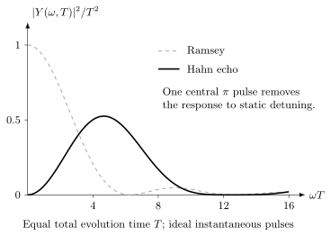
Ramsey and Hahn-echo filter power at the same total evolution time. Echo suppresses the lowest frequencies but increases sensitivity in another band. Integrating over all frequencies gives the same total filter weight for either ideal sign-switching sequence, explaining why white noise cannot be removed by refocusing alone.

Carr–Purcell and CPMG

The Carr–Purcell idea repeats refocusing pulses. For $N$ ideal $\pi$ pulses over total time $T$, a common equally spaced choice places pulses near

$$t_j = \left(j-\frac12\right) \frac{T}{N}, \qquad j=1,\ldots,N.$$

The toggling function changes sign at each $t_j$. The resulting filter has peaks near frequencies set by the pulse spacing, roughly of order

$$\omega \sim \frac{\pi N}{T}.$$

The Meiboom–Gill refinement chooses pulse phases to reduce the accumulation of certain pulse errors for a chosen initial spin component. The name CPMG usually refers to this practical Carr–Purcell–Meiboom–Gill family.

CPMG is useful for suppressing low-frequency dephasing and for noise spectroscopy. It is not a universal cure: it can amplify noise near filter peaks and can fail when pulse errors, finite pulse widths, or transverse relaxation dominate.

Uhrig Sequence Preview

The Uhrig dynamical-decoupling sequence places $N$ pulses at nonuniform times

$$t_j = T \sin^2 \left( \frac{\pi j}{2N+2} \right), \qquad j=1,\ldots,N.$$

For ideal pulses, these times satisfy $\int_0^T t^m y(t)\,dt=0$ for $m=0,\ldots,N-1$. Expanding $e^{i\omega t}$ then gives $Y(\omega,T)=O[T(\omega T)^N]$ at low frequency. Turning this into a high-order short-time bound on decoherence requires sufficiently finite bath spectral moments; it is not a universal ranking for arbitrary spectra. The shortest intervals shrink as $T/N^2$, making finite pulse duration an increasingly important constraint.

The assumptions are important. In experiments with finite pulses, pulse errors, hardware constraints, or noise spectra with broad structure, the best sequence may be CPMG, XY-family sequences, optimized pulses, or something platform-specific rather than Uhrig.

Average Hamiltonian View

The full toggling-frame cycle expansion, including pulse-order commutators, group averaging, time symmetry, and finite-pulse checks, is derived in Average Hamiltonian Theory. Here the construction is used only to connect decoupling with noise suppression.

For a general system–bath coupling

$$H_I = \sum_\alpha A_\alpha\otimes B_\alpha,$$

control transforms system operators in the toggling frame:

$$A_\alpha(t) = U_c^\dagger(t)A_\alpha U_c(t).$$

If the leading time average over a control cycle vanishes,

$$\frac{1}{T_c} \int_0^{T_c} dt\,A_\alpha(t) = 0,$$

then the lowest-order average coupling is removed. This is the intuition behind group-based decoupling sequences.

Higher-order terms depend on commutators at different times. Noncommuting errors require more careful sequences, and fast strong pulses may introduce their own errors.

What Decoupling Can and Cannot Suppress

Dynamical decoupling works best against noise that is slow compared with the pulse spacing and couples in a way the pulses can reverse.

It is naturally effective for:

• low-frequency dephasing noise;
• quasi-static detuning disorder;
• some slowly varying bath fields;
• selected couplings that change sign under the control group;
• sensing protocols that intentionally select a target frequency.

It is limited against:

• broadband Markovian white noise;
• irreversible energy relaxation from high-frequency transverse noise;
• noise above the control bandwidth;
• pulse amplitude, detuning, and phase errors;
• heating or leakage caused by the pulses;
• non-Gaussian noise with rare large events;
• environments with strong backaction or long memory not captured by a simple filter.

For a Markovian Lindblad equation with a fixed relaxation rate, adding pulses does not automatically remove the dissipator. One must model how the control transforms the system-environment coupling before the Markov approximation is made.

Relation to Sensing

Dynamical decoupling is not always used to suppress a signal. In quantum sensing, the sequence is often chosen so that unwanted low-frequency drift is rejected while an oscillating target field passes through the filter.

For a classical signal $s(t)$ coupled through $Z$, the measured phase is

$$\phi_s(T) = \int_0^T dt\,y(t)s(t).$$

Thus the same $y(t)$ that filters noise also defines the signal response. A good sensing sequence separates signal and noise spectrally or by symmetry.

Exercises

Echo Cancels Static Detuning

Let $\xi(t)=\xi_0$ be constant during one experiment. Show that a Hahn echo with one pulse at $T/2$ cancels the accumulated phase.

Solution

The accumulated phase is

$$\varphi(T) = \xi_0 \int_0^T dt\,y_{\mathrm{echo}}(t).$$

For Hahn echo,

$$\int_0^T dt\,y_{\mathrm{echo}}(t) = \int_0^{T/2}dt - \int_{T/2}^{T}dt = \frac{T}{2}-\frac{T}{2} =0.$$

Thus $\varphi(T)=0$ for static detuning.

Ramsey Filter

Starting from $y(t)=1$, derive

$$Y_{\mathrm{Ramsey}}(\omega,T) = \frac{e^{i\omega T}-1}{i\omega}.$$

Solution

By definition,

$$Y_{\mathrm{Ramsey}}(\omega,T) = \int_0^T dt\,e^{i\omega t}.$$

For $\omega\ne0$,

$$\int_0^T dt\,e^{i\omega t} = \frac{e^{i\omega T}-1}{i\omega}.$$

The $\omega\to0$ limit is $T$, showing strong sensitivity to very slow noise.

Echo Filter at Low Frequency

Use

$$Y_{\mathrm{echo}} = \frac{ 2e^{i\omega T/2}-1-e^{i\omega T} } {i\omega}$$

to show that the echo filter suppresses static noise.

Solution

Let $x=\omega T/2$. Then the numerator is

$$2e^{ix}-1-e^{2ix}=-\left(1-e^{ix}\right)^2.$$

For small $x$,

$$1-e^{ix} \approx -ix,$$

so the numerator is of order $x^2$. Therefore

$$Y_{\mathrm{echo}} \propto \frac{\omega^2T^2}{\omega} \sim \omega T^2$$

near $\omega=0$, and the filter power $|Y_{\mathrm{echo}}|^2$ vanishes at zero frequency.

Markovian Limit

Why does a pulse sequence generally fail to improve coherence if the noise is perfectly white and the pulse sequence only changes the sign of the coupling?

Solution

White noise has no long-time memory to refocus. In the filter formula, a flat spectrum gives

$$\chi(T) = \frac12S_0 \int \frac{d\omega}{2\pi} |Y(\omega,T)|^2.$$

Parseval’s identity turns the integral into

$$\int_0^Tdt\,|y(t)|^2.$$

For ideal sign flips, $|y(t)|^2=1$, so this integral remains $T$. The pulses rearrange phases but do not reduce the total exposure to memoryless noise.

References

• H. Y. Carr and E. M. Purcell, “Effects of diffusion on free precession in nuclear magnetic resonance experiments,” Physical Review 94, 630–638 (1954).
• L. Cywiński, R. M. Lutchyn, C. P. Nave, and S. Das Sarma, “How to enhance dephasing time in superconducting qubits,” Physical Review B 77, 174509 (2008). doi:10.1103/PhysRevB.77.174509.
• E. L. Hahn, “Spin echoes,” Physical Review 80, 580–594 (1950).
• D. A. Lidar and T. A. Brun, eds., Quantum Error Correction, Cambridge University Press (2013), chapters on dynamical decoupling.
• S. Meiboom and D. Gill, “Modified spin-echo method for measuring nuclear relaxation times,” Review of Scientific Instruments 29, 688–691 (1958).
• G. S. Uhrig, “Keeping a quantum bit alive by optimized pi-pulse sequences,” Physical Review Letters 98, 100504 (2007). doi:10.1103/PhysRevLett.98.100504.
• L. Viola and S. Lloyd, “Dynamical suppression of decoherence in two-state quantum systems,” Physical Review A 58, 2733–2744 (1998).