Spin and Spinors

Spin is intrinsic angular momentum: it transforms under rotations without being the orbital motion of a small spinning object. Spin-$1/2$ is an especially useful example because two complex amplitudes describe its pure state, three Pauli matrices describe its spin components, and a sphere organizes its measurement probabilities. This chapter connects those descriptions to magnetic precession and then explains what changes for larger spin.

Helpful background. Angular-momentum algebra supplies the commutators and multiplet labels. Rays and global phase explains why a spinor’s overall sign is not an isolated observable.

Enter this chapter

Question	Read next
What makes spin intrinsic angular momentum?	What spin is and spin as angular momentum
How is a two-component state calculated?	Spin-$1/2$ Hilbert space and Pauli matrices
What does a measurement along an axis predict?	Bloch sphere, spin measurements, and Stern–Gerlach revisited
Why do rotations use half-angles?	Spin rotations and the 2π sign
Which direction precesses, and at what rate?	Magnetic fields, Larmor precession, and magnetic moments
What replaces the simple Bloch picture for larger spin?	Higher spin and spin coherent states

Spinors and physical spin components

In the $S_z$ basis, write a normalized spin-$1/2$ state as $|\psi\rangle=\alpha|\uparrow\rangle+\beta|\downarrow\rangle$, with $|\alpha|^2+|\beta|^2=1$. The basis states have $S_z$ eigenvalues $\pm\hbar/2$. The corresponding matrices are

$$S_i=\frac{\hbar}{2}\sigma_i, \qquad \sigma_i\sigma_j=\delta_{ij}I+i\sum_k\epsilon_{ijk}\sigma_k.$$

The Pauli matrices are dimensionless; the spin operators carry angular-momentum units. “Up” and “down” refer to the stated axis, not to an axis-independent property. A spatial wavefunction may also be present: in the elementary nonrelativistic model, the state space is $L^2(\mathbb R^3)\otimes\mathbb C^2$, and total rotations act on both factors through $\mathbf J=\mathbf L+\mathbf S$.

The Bloch direction predicts measurement probabilities

After removing global phase, every pure spin-$1/2$ state can be written

$$|\hat{\mathbf n}\rangle = \cos\frac{\theta}{2}|\uparrow\rangle + e^{i\phi} \sin\frac{\theta}{2}|\downarrow\rangle,$$

where

$$\hat{\mathbf n} = \begin{pmatrix} \sin\theta\cos\phi\\ \sin\theta\sin\phi\\ \cos\theta \end{pmatrix}.$$

This direction is recovered from expectation values:

$$\langle\boldsymbol\sigma\rangle = \hat{\mathbf n}, \qquad \langle\mathbf S\rangle = \frac{\hbar}{2}\hat{\mathbf n}.$$

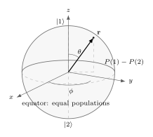
A normalized spin-$1/2$ ray is represented by a point $\hat{\mathbf n}$ on the sphere. The spinor uses half-angles, while the expectation-value direction transforms as an ordinary vector.

The same state has density operator

$$\rho = \frac12 \left( I+\hat{\mathbf n}\cdot\boldsymbol\sigma \right).$$

Mixed spin-$1/2$ states replace $\hat{\mathbf n}$ by a vector $\mathbf r$ with $|\mathbf r|<1$, filling the Bloch ball. That density-operator treatment belongs to Bloch Sphere for Density Operators.

For $s>1/2$, a direction on a sphere no longer specifies every pure state. Spin coherent states form an important sphere inside the larger projective state space, but generic higher-spin states contain additional multipole information.

Measurements use a chosen axis

A spin measurement must specify an axis. Along a unit vector $\hat{\mathbf a}$, the measured observable is

$$S_{\hat a} = \hat{\mathbf a}\cdot\mathbf S = \frac{\hbar}{2} \hat{\mathbf a}\cdot\boldsymbol\sigma.$$

Because

$$(\hat{\mathbf a}\cdot\boldsymbol\sigma)^2=I,$$

the outcomes are $\pm\hbar/2$, with projectors

$$P_\pm^{(\hat a)} = \frac12 \left( I\pm \hat{\mathbf a}\cdot\boldsymbol\sigma \right).$$

For a state with Bloch vector $\mathbf r$,

$$p_\pm = \operatorname{Tr} \left( \rho P_\pm^{(\hat a)} \right) = \frac12 \left( 1\pm\mathbf r\cdot\hat{\mathbf a} \right).$$

As a useful geometric example, prepare the $+\hat{\mathbf n}$ state and measure along $\hat{\mathbf a}$. If the angle between the axes is $\gamma$, then

$$p_+ = \cos^2\frac{\gamma}{2}, \qquad p_- = \sin^2\frac{\gamma}{2}.$$

The overlap of the two spinors gives these half-angle probabilities. Orthogonal laboratory axes have $\gamma=\pi/2$ and therefore give equal probabilities, not deterministic opposite outcomes.

Different components generally do not commute:

$$[S_{\hat a},S_{\hat b}] = i\hbar (\hat{\mathbf a}\times\hat{\mathbf b}) \cdot\mathbf S.$$

Thus preparing an eigenstate along one axis usually destroys sharpness along another. The general rules for Born probabilities, selective update, and nonselective measurement are developed in Core Formalism; this chapter supplies their spin-$1/2$ realization.

An ideal Stern–Gerlach analyzer correlates the two spin projections with distinguishable paths. Preparing $+z$, selecting the $+x$ output of an $x$ analyzer, and measuring $z$ again gives equal $+z$ and $-z$ probabilities in that selected ensemble. The selection prepares a new state. Ignoring the outcome instead gives a mixture, which can have the same probabilities for one later measurement but differ for others. Stern–Gerlach revisited connects the matrix calculation to the apparatus, while the historical experiment explains the silver-atom setting.

Spinor rotations and vector rotations

The unitary operator for an active rotation by angle $\theta$ about $\hat{\mathbf n}$ is

$$U(\hat{\mathbf n},\theta) = \exp\!\left( -\frac{i\theta}{\hbar} \hat{\mathbf n}\cdot\mathbf S \right).$$

For spin $1/2$,

$$U(\hat{\mathbf n},\theta) = \exp\!\left( -\frac{i\theta}{2} \hat{\mathbf n}\cdot\boldsymbol\sigma \right).$$

Using $(\hat{\mathbf n}\cdot\boldsymbol\sigma)^2=I$ gives

$$U(\hat{\mathbf n},\theta) = \cos\frac{\theta}{2}\,I -i\sin\frac{\theta}{2} \hat{\mathbf n}\cdot\boldsymbol\sigma.$$

The spinor carries the half-angle, but its Bloch vector rotates through the physical angle $\theta$. If $\mathcal R\in SO(3)$ is the corresponding vector rotation, then

$$U (\mathbf a\cdot\boldsymbol\sigma) U^\dagger = (\mathcal R\mathbf a) \cdot\boldsymbol\sigma.$$

This relation is a practical bridge between $SU(2)$ matrix calculations and ordinary three-dimensional geometry. It also makes the two-to-one map explicit: $U$ and $-U$ induce the same $SO(3)$ rotation of Bloch vectors.

A full rotation can create a relative phase

For spin $1/2$, one full physical turn gives

$$U(\hat{\mathbf n},2\pi)=-I,$$

whereas two full turns give

$$U(\hat{\mathbf n},4\pi)=I.$$

More generally, the central element associated with a $2\pi$ rotation acts on a spin-$s$ irreducible multiplet as

$$U_s(2\pi) = (-1)^{2s}I.$$

Integer-spin state vectors return after $2\pi$; half-integer-spin vectors acquire a minus sign. This is a global representation-theoretic distinction, not a consequence visible from the infinitesimal commutators alone.

The sign does not change an isolated ray because

$$|\psi\rangle \sim e^{i\alpha}|\psi\rangle.$$

In particular, $|\psi\rangle$ and $-|\psi\rangle$ represent the same pure state. The sign becomes observable when it is relative to another coherent amplitude. If only one arm of an interferometer applies a $2\pi$ spin rotation, then schematically

$$\begin{aligned} \frac{|a\rangle+|b\rangle}{\sqrt2} \otimes|\chi\rangle &\longmapsto \\ \frac{|a\rangle-|b\rangle}{\sqrt2} \otimes|\chi\rangle. \end{aligned}$$

Recombining the paths detects the changed relative phase. The Bloch sphere cannot display this sign because $U$ and $-U$ act identically on the Bloch vector.

Magnetic precession requires coherence

For an effective moment $\boldsymbol\mu=\gamma\mathbf S$ in a static field $\mathbf B=B_0\hat{\mathbf z}$, with $B_0>0$,

$$H=-\gamma B_0 S_z,\qquad E_{\pm z}=\mp\frac{\gamma\hbar B_0}{2}.$$

The splitting is $\hbar|\gamma|B_0$, but the lower state depends on the sign of $\gamma$. For an electron, the magnetic moment is opposite to spin, so “aligned is lower” must specify whether it refers to the moment or the spin.

The spin equation is

$$\frac{d\langle\mathbf S\rangle}{dt} =\gamma\langle\mathbf S\rangle\times\mathbf B.$$

An energy eigenstate has a stationary Bloch vector. A state with transverse coherence precesses because its two energy components acquire a changing relative phase. Exercise 3 fixes the direction for the stated sign convention. The magnetic-moment article also distinguishes orbital and spin $g$ factors and anisotropic effective moments.

Higher spin contains more than a direction

An irreducible spin-$s$ space has dimension $2s+1$. Rotating $|s,s\rangle$ generates the coherent states $|\hat{\mathbf n};s\rangle$, with $\langle\mathbf S\rangle=\hbar s\hat{\mathbf n}$. For $s=1/2$ every pure state is of this form. For $s>1/2$, it is only a two-parameter subset of the full pure-state space.

For example, spin-one $|1,0\rangle$ has $\langle\mathbf S\rangle=0$, but it is pure, not maximally mixed. Its second moments distinguish an axis: $\langle S_z^2\rangle=0$ and $\langle S_x^2\rangle=\langle S_y^2\rangle=\hbar^2$. Higher moments therefore carry information that the mean spin vector omits. See higher spin systems for the matrix construction and spin coherent states for the semiclassical limit.

Exercises

1. Show that the arbitrary-axis operators

$$P_\pm = \frac12 \left( I\pm\hat{\mathbf n}\cdot\boldsymbol\sigma \right)$$

are orthogonal projectors that sum to the identity.

Solution

For a unit vector $\hat{\mathbf n}$, the Pauli product identity gives

$$(\hat{\mathbf n}\cdot\boldsymbol\sigma)^2=I.$$

Therefore

$$\begin{aligned} P_\pm^2 &= \frac14 \left( I \pm2\hat{\mathbf n}\cdot\boldsymbol\sigma +I \right) \\ &= P_\pm. \end{aligned}$$

The sum is $P_++P_-=I$, and

$$P_+P_- = \frac14 \left[ I-(\hat{\mathbf n}\cdot\boldsymbol\sigma)^2 \right] = 0.$$

Thus the two ranges are orthogonal and complete.

2. Consider

$$|\psi\rangle = \frac{\sqrt3}{2}|\uparrow\rangle + \frac{i}{2}|\downarrow\rangle.$$

Find its Bloch vector and the probability of obtaining $+\hbar/2$ in an $S_x$ measurement.

Solution

For a normalized spinor $(\alpha,\beta)^T$,

$$\mathbf r = \begin{pmatrix} 2\operatorname{Re}(\alpha^*\beta)\\ 2\operatorname{Im}(\alpha^*\beta)\\ |\alpha|^2-|\beta|^2 \end{pmatrix}.$$

Here $\alpha=\sqrt3/2$ and $\beta=i/2$, so

$$\mathbf r = \begin{pmatrix} 0\\ \sqrt3/2\\ 1/2 \end{pmatrix}.$$

For an $x$-axis measurement,

$$p(+x) = \frac12(1+r_x) = \frac12.$$

3. A spin-$1/2$ state initially points along $+x$ and evolves under

$$H=-\gamma B_0S_z.$$

For $\gamma B_0>0$, find its Bloch vector as a function of time and state its initial direction of motion.

Solution

Let $\omega=\gamma B_0>0$. The precession equations give

$$\mathbf r(t) = \begin{pmatrix} \cos\omega t\\ -\sin\omega t\\ 0 \end{pmatrix}.$$

At $t=0$, $d\mathbf r/dt=(0,-\omega,0)$, so the Bloch vector initially moves from $+x$ toward $-y$. Replacing $\gamma$ by a negative value reverses the sense of precession without changing the positive frequency magnitude $|\gamma|B_0$.

References

• C. Cohen-Tannoudji, B. Diu, and F. Laloë, Quantum Mechanics, Wiley, 1977.
• C. J. Foot, Atomic Physics, Oxford University Press, 2005.
• D. J. Griffiths and D. F. Schroeter, Introduction to Quantum Mechanics, 3rd ed., Cambridge University Press, 2018.
• B. C. Hall, Lie Groups, Lie Algebras, and Representations: An Elementary Introduction, 2nd ed., Springer, 2015.
• A. M. Perelomov, Generalized Coherent States and Their Applications, Springer, 1986.
• H. Rauch and S. A. Werner, Neutron Interferometry: Lessons in Experimental Quantum Mechanics, 2nd ed., Oxford University Press, 2015.
• J. J. Sakurai and J. Napolitano, Modern Quantum Mechanics, 3rd ed., Cambridge University Press, 2020.
• R. Shankar, Principles of Quantum Mechanics, 2nd ed., Springer, 1994.