Stern–Gerlach Experiment

The Stern–Gerlach experiment sends a collimated beam of neutral atoms through an inhomogeneous magnetic field. Instead of forming a continuous vertical smear on a detector, the beam splits into separated components. Real deposits have finite widths and depend on collimation and the atoms’ speed distribution.

Today the experiment is a standard entrance to spin and two-outcome quantum measurements. Historically, the original 1922 silver-atom experiment was interpreted as evidence for directional quantization before the modern electron-spin formalism was in place. Both statements matter: the experiment is a clean modern prototype, but the original interpretation was not simply “they measured free electron spin.”

Atomic Beam Setup

The apparatus has four essential parts:

• an oven that emits neutral silver atoms,
• collimating slits that form a narrow beam,
• an inhomogeneous magnetic field,
• a detector plate where the beam deposits silver.

Neutral atoms were crucial. A charged beam in a magnetic field would experience a Lorentz force depending on its velocity. A neutral atom avoids that dominant charge deflection, while its magnetic moment can still couple to the field gradient.

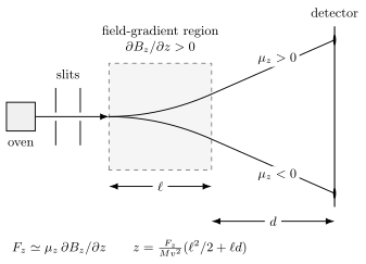
The idealized trajectories show how a field gradient converts magnetic-moment projection into spatial deflection, including a drift region after the magnet. The original apparatus collected silver immediately after the magnet and produced extended split deposits rather than pointlike spots.

Magnetic Field Gradient

A magnetic moment $\boldsymbol\mu$ in a magnetic field has interaction energy

$$U = - \boldsymbol\mu\cdot\mathbf B.$$

The force is the gradient of $\boldsymbol\mu\cdot\mathbf B$. In the simplest geometry, the vertical force is approximated by

$$F_z \simeq \mu_z \frac{\partial B_z}{\partial z}.$$

This approximation assumes the moment follows the local field adiabatically and that one gradient dominates. More generally, an internal energy branch $E_a(\mathbf r)$ gives force $\mathbf F_a=-\nabla E_a$. Real magnets also have transverse field components; the simple formula is a local beam model.

The field must be nonuniform. A uniform magnetic field can exert a torque on a magnetic moment, but it does not by itself separate a neutral beam into spatial components. The gradient makes different magnetic-moment projections follow different trajectories.

Classical Expectation

In a classical picture, magnetic moments can point in a continuum of orientations. If the beam contains atoms with many orientations, then the projection

$$\mu_z = \mu\cos\theta$$

can take a continuous range of values. The detector should show a continuous vertical distribution, broadened by the range of possible forces.

That is not what the experiment found. The silver beam separated into discrete components. The result challenged the idea that microscopic angular-momentum-like quantities simply have arbitrary classical orientations.

Observed Splitting

Gerlach and Stern compared deposits with the field off and on. Without the field, the slit produced a narrow stripe; with the field, the stripe separated into two bands, with no detected undeflected component. The authors also reported broader bands from the velocity distribution and unequal deflections because the gradient was stronger near the sharp pole. These controls and finite-width features, documented in their 1922 report in English translation, distinguish the observed pattern from the schematic two trajectories.

In the original historical context, this was evidence for directional, or “space,” quantization: only certain projections of the relevant angular momentum along the apparatus axis were allowed.

Modern language is sharper. The apparatus orientation defines a component of an angular momentum or spin-like degree of freedom. The measurement outcomes are eigenvalues of that component, not arbitrary pre-existing classical directions. The original silver-atom experiment is especially useful because the ground-state silver atom is well approximated, for this purpose, by an effective two-state magnetic degree of freedom associated with its valence electron.

Space Quantization

“Space quantization” does not mean that physical space becomes a lattice. It means that the projection of angular momentum along the magnetic-field direction takes discrete values.

For angular momentum $J$, the modern eigenvalue statement is

$$J_z\lvert j,m\rangle = \hbar m\lvert j,m\rangle,$$

where

$$m = -j,-j+1,\ldots,j.$$

For a two-state spin-$1/2$ idealization,

$$S_z\lvert +z\rangle = \frac{\hbar}{2}\lvert +z\rangle, \qquad S_z\lvert -z\rangle = - \frac{\hbar}{2}\lvert -z\rangle.$$

Those two eigenvalues correspond to two ideal output beams for a measurement along $z$, with the spatial order determined by the magnetic-moment sign and field gradient.

Connection to Spin

Electron spin was proposed after the original Stern–Gerlach experiment. The modern interpretation of the silver-atom result uses the fact that silver has one relevant unpaired valence electron in an $s$ state, so the effective magnetic degree of freedom is closely tied to spin rather than ordinary orbital angular momentum.

For a spin magnetic moment, an effective coupling is often written

$$\boldsymbol\mu = \gamma\mathbf S,$$

where the constant $\gamma$ depends on the particle and sign convention. A Stern–Gerlach magnet then correlates spin-component eigenstates with spatial paths:

$$\lvert +z\rangle \longrightarrow \text{upper beam}, \qquad \lvert -z\rangle \longrightarrow \text{lower beam}.$$

The upper/lower assignment above assumes $\gamma\,\partial B_z/\partial z>0$. For an electron-like silver moment, $\gamma<0$; with $\partial B_z/\partial z>0$, the $+z$ spin branch deflects downward. Labeling the upper beam “spin up” without a magnetic-moment sign convention is therefore unsafe.

The silver ground state has a closed core and a valence electron with $L=0$ and $J=1/2$. Nuclear spin and hyperfine coupling add structure; the two-beam picture treats the dominant electronic moment in the regime where those corrections do not resolve extra branches.

From force to a detector displacement

Let the magnet length be $\ell$, the following drift distance be $d$, the atomic mass be $M$, and the approximately constant longitudinal speed be $v$. Take the incoming transverse position and velocity to be zero. A branch feeling constant transverse force $F_z$ spends $\ell/v$ in the magnet and leaves it with

$$z_{\mathrm{exit}}=\frac{F_z\ell^2}{2Mv^2}, \qquad v_{z,\mathrm{exit}}=\frac{F_z\ell}{Mv}.$$

During the drift time $d/v$, it acquires the additional displacement $v_{z,\mathrm{exit}}d/v$. Thus the detector position is

$$z=\frac{F_z}{Mv^2}\left(\frac{\ell^2}{2}+\ell d\right).$$

The first term is the accelerated motion inside the magnet; the second is free drift with the acquired transverse velocity. Slower atoms deflect farther, explaining one source of finite spot width. This estimate assumes small deflections, a nearly constant gradient over the trajectories, and negligible fringe-field forces.

For an illustrative silver beam, use $M=1.79\times10^{-25}\,\mathrm{kg}$, $\lvert\mu_z\rvert\simeq\mu_B=9.27\times10^{-24}\,\mathrm{J/T}$, $v=500\,\mathrm{m/s}$, $\ell=3.0\,\mathrm{cm}$, $d=10\,\mathrm{cm}$, and $\partial B_z/\partial z=10^3\,\mathrm{T/m}$. The mass and magnetic-moment scale are rounded from the NIST data listed below; the speed and geometry are chosen for this example. Then

$$\lvert F_z\rvert=9.27\times10^{-21}\,\mathrm N, \qquad \lvert z\rvert\simeq0.715\,\mathrm{mm}, \qquad \Delta z_{\mathrm{beams}}=2\lvert z\rvert\simeq1.43\,\mathrm{mm}.$$

The exit angle is only $\lvert v_{z,\mathrm{exit}}\rvert/v\simeq0.0062$, consistent with the small-angle kinematics. For the electron-like moment, the $m_s=+1/2$ branch has $\mu_z<0$ and reaches $z\simeq-0.715\,\mathrm{mm}$. Resolving the two branches additionally requires their widths to be small compared with the separation. These numbers illustrate the model; reproducing the historical deposits requires the actual field profile, slit geometry, and velocity distribution.

Modern Two-Level Interpretation

For a spin-$1/2$ system, a measurement axis $\hat{\mathbf n}$ corresponds to the operator

$$S_{\hat{\mathbf n}} = \frac{\hbar}{2} \boldsymbol\sigma\cdot\hat{\mathbf n},$$

with outcomes

$$\pm\frac{\hbar}{2}.$$

If the incoming spin state is $\lvert\psi\rangle$, the probability of the $+\hat{\mathbf n}$ output is

$$P(+\hat{\mathbf n}) = \lvert \langle +\hat{\mathbf n}\vert\psi\rangle \rvert^2.$$

Changing the magnet orientation changes the measured operator. A state that is definite along $z$ is generally not definite along $x$. This is why sequential Stern–Gerlach experiments are so useful: a $z$ analyzer, followed by an $x$ analyzer, followed by another $z$ analyzer exposes noncommuting measurement axes and state update.

The detailed spinor formalism is developed in Spin-1/2 Hilbert Space, Pauli Matrices, and Stern–Gerlach Revisited. The measurement idealization belongs in Projective Measurement and Sequential Measurements.

For the historical projection language that grew out of the experiment, see Space Quantization.

Common Misconceptions

• The original experiment was not a literal free-electron spin measurement.
• The two spots are not evidence that each atom carried a small classical arrow with a pre-existing orientation along every possible axis.
• A Stern–Gerlach device does not measure “spin” without specifying an axis; the magnet geometry defines the component.
• The word “up” names an eigenstate relative to an apparatus axis, not an absolute direction carried around by the particle.
• The absence of a continuous smear is the key historical shock; the modern noncommuting-axis lesson requires sequential measurements.

Exercises

1. Explain why an inhomogeneous magnetic field is required for beam splitting.

Solution

The force on a neutral magnetic moment is obtained from the spatial gradient of its interaction energy. In the simplified geometry, $F_z\simeq\mu_z\,\partial B_z/\partial z$. If the field is uniform, $\partial B_z/\partial z=0$, so there is no Stern–Gerlach separation of the neutral beam, even though the magnetic moment may experience a torque.

2. In the numerical beam example, what happens to the full beam separation if the longitudinal speed doubles? What happens if only the field gradient reverses, while the quantization axis and branch magnetic moments remain fixed?

Solution

Both the time in the magnet and the drift time decrease when $v$ increases. Consequently $z\propto v^{-2}$, and doubling $v$ reduces the full separation from $1.43\,\mathrm{mm}$ to about $0.357\,\mathrm{mm}$. Reversing only the gradient changes the sign of each branch force and displacement, so the branches exchange positions without changing the magnitude of their separation. Reversing the entire magnetic field can also change the local quantization axis; that is a different operation from the fixed-axis comparison here.

3. A spin-$1/2$ system is prepared in $\lvert +z\rangle$. It is then measured along $x$, and the $+x$ output is selected. A final measurement is made along $z$. What are the final $z$ probabilities?

Solution

After selecting the $+x$ output, the state is $\lvert +x\rangle$. In the $z$ basis,

$$\lvert +x\rangle = \frac{1}{\sqrt2} \left( \lvert +z\rangle+\lvert -z\rangle \right).$$

Therefore the final $z$ measurement gives

$$P(+z) = \frac{1}{2}, \qquad P(-z) = \frac{1}{2}.$$

These are probabilities conditional on passing the $+x$ selection. Half of the initial $+z$ beam passes that selection, so each final $z$ output contains one quarter of the atoms entering the $x$ analyzer, assuming ideal transmission and detection. The intermediate selection changes the state relative to the original $z$ preparation.

References

• C. Cohen-Tannoudji, B. Diu, and F. Laloë, Quantum Mechanics, Wiley, 1977.
• B. Friedrich and D. Herschbach, “Stern and Gerlach: How a Bad Cigar Helped Reorient Atomic Physics,” Physics Today 56, 53-59 (2003), DOI: 10.1063/1.1650229.
• W. Gerlach and O. Stern, “Der experimentelle Nachweis der Richtungsquantelung im Magnetfeld,” Zeitschrift für Physik 9, 349-352 (1922), DOI: 10.1007/BF01326983. English translation by M. Bauer, 2023.
• National Institute of Standards and Technology, CODATA Recommended Values of the Fundamental Physical Constants: 2022, and “Silver,” NIST Chemistry WebBook, SRD 69. Sources for the rounded Bohr magneton and atomic mass used in the estimate.
• J. J. Sakurai and J. Napolitano, Modern Quantum Mechanics, 3rd ed., Cambridge University Press, 2020.