Noise, Channels, and Error Mitigation

Quantum noise changes preparations, gates and measurements. A useful model must predict the particular experiment we want to perform, including its timing and neighboring operations. Error mitigation then tries to infer selected ideal results from noisy data; it does not generally restore an unknown quantum state.

This chapter connects channel mathematics to circuit behavior. Start with how errors accumulate, learn which channel descriptions capture that behavior, and then compare interventions through both their remaining bias and their statistical uncertainty.

Helpful background. The circuit model defines preparations, gates and measurement outcomes. Quantum channels and noise introduces completely positive maps and conditional operations.

Enter this chapter

For a first reading, follow Noise in Quantum Information, Common Noise Models, then Error Mitigation Overview. If you are translating formulas into a simulation, start instead with Quantum Channels for QI.

Three distinctions will recur:

• A fitted channel describes input–output behavior. It need not identify the unique physical cause.
• Agreement for one measurement does not imply agreement for every circuit.
• A smaller bias can come with larger variance, more rejected runs or additional calibration.

One-step agreement can hide different accumulation

Prepare $\lvert0\rangle$ and compare a coherent unwanted rotation $U_\delta=e^{-i\delta X/2}$ with an independent random $X$ error of probability $p=\sin^2(\delta/2)$ at every step. Their one-step computational-basis flip probabilities agree.

After $m$ repetitions, however, the probabilities of still measuring zero are

$$\begin{aligned} P_{\mathrm{coh}}(0;m)&=\cos^2(m\delta/2),\\ P_{\mathrm{rand}}(0;m)&=\frac{1+(1-2p)^m}{2}. \end{aligned}$$

The coherent rotations add their angles. Independent flips combine through the parity of the number of errors. For $\delta=0.02$ radians and $m=50$, the two probabilities are approximately $0.770151$ and $0.995025$. The same one-step observation therefore predicts neither long-circuit result without further information.

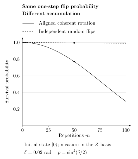
Both models have the same one-step flip probability, but their complete channels differ. The coherent model keeps the same rotation angle and axis on every repetition; the stochastic model draws independent flips. Changing those temporal assumptions changes the curves.

Experiments can distinguish the models by varying sequence length, input axis or pulse order. Spectator activity and acquisition time can also change the response; context-dependent experiments test those possibilities Rudinger et al. (2019).

Decide what the model must describe

For a fixed experiment, outcome probabilities take the form

$$p(y\mid x)=\operatorname{Tr}\!\left[M_y\mathcal E(\rho_x)\right].$$

Here $\rho_x$ describes the actual preparation, $\mathcal E$ the process, and $M_y$ the measurement effect. Observed discrepancies can involve all three. Repeating an experiment more often reduces counting uncertainty, but cannot distinguish two models that predict exactly the same probabilities.

A deterministic channel is appropriate when the chosen input states admit one completely positive trace-preserving map in the specified context. A selected measurement outcome is instead a trace-nonincreasing operation; its trace gives its probability. Keep that probability when conditioning. For leakage, include the levels outside the computational subspace before projecting onto retained outcomes.

Kraus, Choi and transfer matrices are alternative descriptions, not distinct physical mechanisms. One-time channel descriptions also do not determine all multitime responses. Interventions during an evolution can reveal memory absent from a fitted endpoint channel Pollock et al. (2018). Changing experimental conditions is therefore often more informative than fitting another scalar “error rate.”

What mitigation improves

Mitigation commonly estimates an ideal expectation by combining results from noisy experiments. The review by Cai et al. (2023) compares the methods and their assumptions. A linear estimator has

$$\hat\mu=\sum_j w_j\hat\mu_j, \qquad \operatorname{Var}(\hat\mu)=\mathbf w^{\mathsf T}\Sigma\mathbf w,$$

where $\Sigma$ is the covariance matrix of the measured means. Negative weights can cancel leading bias while amplifying uncertainty. If the weights were learned from finite calibration data, their uncertainty also contributes.

For example, extrapolation weights $(3,-3,1)$ at noise scales $(1,2,3)$ preserve a constant and cancel linear and quadratic terms. Their absolute sum is seven. With independent, equal single-shot variances and optimal allocation of a fixed total shot budget, the variance is 49 times the corresponding single-setting variance. This factor does not establish that the physical experiment actually follows the assumed noise-scaling family.

Postselection has a different cost. Accepting a fraction $a$ of independent stationary attempts requires $N/a$ attempts on average to obtain $N$ accepted records. The selected quantity is generally conditional on acceptance. A filter can miss errors that preserve the checked symmetry.

Control, mitigation and correction can be combined, but do different work. Dynamical decoupling changes the physical evolution; readout inversion and extrapolation change an estimate; error correction uses redundant encoding and recovery to protect logical information. Continue to why quantum error correction is possible when protecting unknown states is the goal.

Choose a page by the question

Describe the process

Question	Read
Which mechanisms and diagnostics matter?	Noise in Quantum Information
Which representation makes a calculation simplest?	Quantum Channels for QI
How do representations and environment descriptions agree?	Kraus, Choi, and Stinespring Views
Which model and parameter convention should I use?	Common Noise Models
When is a Pauli approximation suitable?	Pauli Noise and Depolarizing Channels
How do populations and coherences decay?	Dephasing and Amplitude Damping
What happens outside the code space or during neighboring operations?	Leakage and Crosstalk
Can I separate preparation and detector errors?	SPAM Errors
When does repeating a channel fail to predict a sequence?	Markovian and Non-Markovian Noise

Improve a result

Question	Read
Which intervention fits my observable and resources?	Error Mitigation Overview
Can I correct a terminal detector response?	Measurement Error Mitigation
Can measurements at larger noise infer an ideal intercept?	Zero-Noise Extrapolation
How do signed mixtures estimate an ideal operation?	Probabilistic Error Cancellation
Which errors does a known symmetry detect?	Symmetry Verification
Can pulses suppress the relevant coupling?	Dynamical Decoupling
When is the sampling or calibration cost prohibitive?	Limits of Error Mitigation

For practical calculations, noise simulation develops numerical propagation. Device characterization explains how to test whether a fitted model predicts measurements beyond those used to fit it.

Exercises

1. Separate preparation, process and measurement

Take $\rho_s=(I+sZ)/2$, a channel sending $Z$ polarization to $\lambda$ times itself, and measurement effect $M_0=(I+mZ)/2$, with all three parameters in $[0,1]$. Find $p_0$. Compare $(s,\lambda,m)=(0.8,0.75,0.9)$ and $(0.9,0.8,0.75)$.

Solution

Using $\operatorname{Tr}Z=0$ and $\operatorname{Tr}Z^2=2$ gives $p_0=(1+m\lambda s)/2$. Both triples give $p_0=0.77$. Arbitrarily many repetitions of this single experiment cannot separate these explanations. Additional trusted settings or sequence constraints are needed; a more precise estimate of the same probability is insufficient.

2. Follow an aligned coherent error

Set $\delta=0.02$ and $m=50$. Reproduce the two survival probabilities. What changes if the coherent rotation is followed by its exact inverse rather than another rotation of the same sign?

Solution

The coherent result is $\cos^2(0.5)\approx0.770151$. For $p=\sin^2(0.01)$, independent flips give $[1+(1-2p)^{50}]/2\approx0.995025$. The inverse pair obeys $U_{-\delta}U_\delta=I$ and cancels perfectly in this ideal error-only model. Two independent random flips instead cancel only when their parity is even, with probability $(1-p)^2+p^2$. The inverse-pair statement assumes the second operation really reverses the same error; it is not a guarantee for imperfect control pulses.

3. Check cancellation and the price in variance

For scales $k=(1,2,3)$ and weights $w=(3,-3,1)$, check cancellation through quadratic order. If each setting has independent single-shot variance $v$, compare equal shot allocation with the optimal allocation at fixed total count $N$. What happens to a cubic term?

Solution

The weighted moments of orders zero, one and two are $1,0,0$. Equal allocation $N_j=N/3$ gives variance $57v/N$. Minimizing $\sum_jw_j^2v/N_j$ with $\sum_jN_j=N$ gives $N_j=N|w_j|/7$, up to integer rounding, and variance $49v/N$. The cubic moment is $3-3(8)+27=6$, so a term $c_3\lambda^3k^3$ leaves $6c_3\lambda^3$. Correlations, unequal variances, uncertain weights and inaccurate physical scaling require additional analysis.

References

• Z. Cai, R. Babbush, S. C. Benjamin, S. Endo, W. J. Huggins, Y. Li, J. R. McClean, and T. E. O’Brien, “Quantum Error Mitigation,” Reviews of Modern Physics 95, 045005 (2023), doi:10.1103/RevModPhys.95.045005.
• F. A. Pollock, C. Rodríguez-Rosario, T. Frauenheim, M. Paternostro, and K. Modi, “Non-Markovian Quantum Processes: Complete Framework and Efficient Characterization,” Physical Review A 97, 012127 (2018), doi:10.1103/PhysRevA.97.012127.
• K. Rudinger, T. Proctor, D. Langharst, M. Sarovar, K. Young, and R. Blume-Kohout, “Probing Context-Dependent Errors in Quantum Processors,” Physical Review X 9, 021045 (2019), doi:10.1103/PhysRevX.9.021045.