Noise in Quantum Information

Noise is the difference between an intended quantum experiment and its physical implementation. It includes environmental decoherence, but also an isolated qubit rotated through the wrong angle, population in unwanted levels, and a detector that reports the wrong result. These mechanisms need different models and different remedies. This page explains how to distinguish them and why a single error percentage seldom predicts an entire circuit.

Helpful background. The circuit model defines the intended operations; density operators describe mixtures and reduced states. Quantum channels provide the completely positive maps used below.

Noise changes experimental probabilities

Suppose input label $x$ selects a preparation $\rho_x$, the device applies a channel $\mathcal E$, and a measurement has effects $M_y$. Its predictions are

$$p(y\mid x,t,c)=\operatorname{Tr}\!\left[ M_{y,t,c}\,\mathcal E_{t,c}(\rho_{x,t,c})\right].$$

Here $t$ is the acquisition time and $c$ describes the circuit context: neighboring drives, simultaneous measurements, idle intervals and earlier pulses. A fixed channel is useful only when those dependencies can be ignored for the experiment being predicted. We assume a common preparation domain supports the channel description; arbitrary initial system–environment correlations need not admit one channel for all preparations.

An observed discrepancy can come from preparation, evolution, measurement, or several together. For example, if preparation produces Bloch polarization $s$, the gate shrinks it by $\lambda$, and readout has contrast $m$, the measured polarization is $s\lambda m$. One number does not determine all three factors. The physical boundary also matters: populating a third atomic level is an error for a qubit gate even if the full three-level motion is perfectly unitary.

The following categories overlap. Crosstalk can cause a coherent phase; drift can turn that phase into an apparent mixture when many runs are averaged.

Mechanism	What changes	A useful distinction
Coherent control error	amplitudes evolve under the wrong unitary	aligned rotations can accumulate before probabilities are formed
Relaxation and dephasing	populations or reduced-state coherences decay	a lifetime is specific to a state, basis and experiment
Leakage or loss	population leaves the physical computational space	a detected erasure differs from hidden loss
Crosstalk	a process depends on activity elsewhere	isolated-gate performance may not transfer to parallel gates
Preparation and readout error	the input state or measurement differs from the intended one	an output bias need not be a gate error
Drift and memory	parameters change, or successive errors are dependent	one-step data need not predict a long sequence

Coherent errors and stochastic faults accumulate differently

A systematic overrotation is a unitary error. For example, a nominal identity cycle might instead apply

$$V_\epsilon=e^{-i\epsilon X/2}.$$

Starting in $|0\rangle$ and repeating the same error $L$ times gives

$$\begin{aligned} V_\epsilon^L&=e^{-iL\epsilon X/2},\\ P(1)&=\sin^2(L\epsilon/2) \simeq L^2\epsilon^2/4. \end{aligned}$$

The approximation requires $L|\epsilon|\ll1$. Angles add first, so this probability grows quadratically at short times. It eventually oscillates; there is no unlimited quadratic growth. Other ideal gates can rotate the error axis. In particular, $ZV_\epsilon Z=V_\epsilon^\dagger$, so an ideal refocusing sequence can cancel this error rather than amplify it.

Compare this with independently applying $X$ with probability $p=\sin^2(\epsilon/2)$ on each cycle. Both models have the same one-cycle $Z$-basis flip probability on $|0\rangle$, but the stochastic model gives

$$P(1)=\frac{1-(1-2p)^L}{2}.$$

This is the probability of an odd number of flips: two $X$ errors cancel. By contrast, the probability of at least one fault is $1-(1-p)^L\simeq Lp$ for $Lp\ll1$. Counting faults and predicting an output error are different calculations. The chapter’s accumulation plot shows the coherent and stochastic results on common axes.

An incoherent reduced description can arise from entanglement with an environment or from averaging over unobserved classical variables. The same detuning may be coherent within one shot and produce dephasing across shots. Decoherence is loss of phase coherence in a specified reduced description; a wrong unitary alone is not decoherence. Dephasing and dissipation also need not change populations in the same way.

Average infidelity and worst-case distance

For a CPTP map on a fixed $d$-dimensional space and an ideal unitary $U$, define

$$\begin{aligned} F_{\rm avg}(\mathcal E,U) &=\int d\psi\,\langle\psi|U^\dagger \mathcal E(|\psi\rangle\langle\psi|)U|\psi\rangle,\\ r&=1-F_{\rm avg},\\ D_\diamond&=\tfrac12\|\mathcal E-\mathcal U\|_\diamond. \end{aligned}$$

The integral averages uniformly over pure inputs. The diamond distance instead maximizes output distinguishability, allowing an input entangled with an unchanged reference. With equal prior probabilities, the best one-use success probability for distinguishing the two channels is $(1+D_\diamond)/2$.

For the qubit overrotation above, and for the independent Pauli channel $(1-p)\rho+pX\rho X$ matched by $p=\sin^2(\epsilon/2)$,

Error channel	Average infidelity	Diamond distance from the identity
coherent rotation	$r=2p/3$	$D_\diamond=\sqrt p$
stochastic Pauli flip	$r=2p/3$	$D_\diamond=p$

For a pure qubit with Bloch component $x$, the rotation’s survival probability is $1-p+px^2$. Averaging $x^2$ over the sphere gives $1/3$, explaining $r=2p/3$. An input perpendicular to the rotation axis attains output trace distance $\sqrt p$. For the Pauli channel, convexity bounds that distance by $p$, and $|0\rangle$ attains it. An ancillary system cannot improve either maximum. Thus the same average infidelity can conceal quite different worst-case behavior (Kueng et al.).

Average infidelity does give bounds; it is not devoid of worst-case information:

$$\frac{d+1}{d}r\ \leq\ D_\diamond \ \leq\ \min\!\left\{1,\sqrt{d(d+1)r}\right\}.$$

These bounds assume the stated fixed-space CPTP channel and unitary target. They do not make a calibration valid in a different circuit context, turn a trace-decreasing postselected map into a channel, or account for omitted leakage levels. Benchmark decay parameters also require a model before they can be interpreted as $r$; gate-dependent noise complicates that interpretation (Proctor et al.).

Relaxation and dephasing times

For a two-level system, $T_1$ describes longitudinal population relaxation; $T_2$ describes transverse coherence decay. In the Markovian model with independent energy relaxation and pure dephasing,

$$\frac1{T_2}=\frac1{2T_1}+\frac1{T_\phi},\qquad T_2\leq2T_1.$$

The factor $1/2$ reflects that an amplitude decays at half the corresponding population-decay rate. This relation assumes compatible exponential rates for the same operating conditions. It is not a definition for arbitrary driven, multilevel or non-Markovian dynamics. Ramsey measurements often quote $T_2^*$, which includes slowly varying frequency offsets; echo can remove some of that broadening. Decoherence timescales explains the experiments and assumptions.

A gate much shorter than $T_1$ can still have a substantial overrotation, unwanted coupling or leakage. A lifetime alone therefore cannot predict gate fidelity.

Leakage, loss and the computational space

Let $P$ project onto the physical computational space, with input $\rho=P\rho P$. For trace-preserving evolution on the full space,

$$\ell(\rho)=\operatorname{Tr}[(I-P)\mathcal E(\rho)] =1-\operatorname{Tr}[P\mathcal E(\rho)]$$

is the output leakage probability. Higher transmon levels, unwanted atomic states or a photonic vacuum outside a fixed-photon encoding are examples. The retained map $P\mathcal E(\rho)P$ is generally trace decreasing; its trace is the acceptance probability, not a normalization to discard silently.

Distinguish this physical space from a smaller error-correcting code. For the repetition code spanned by $|000\rangle,|111\rangle$, an $X$ error on one qubit leaves the code while remaining inside the three-qubit Hilbert space. That is an ordinary correctable error, not physical leakage. The carrier and encoding hierarchy makes this distinction explicit.

Return from a leaked level, often called seepage, need not restore the unknown state or its entanglement. Likewise, detecting a lost dual-rail photon reveals an erasure location, but reloading a photon alone cannot reconstruct the lost logical amplitudes. See erasure and loss channels and leakage and crosstalk for channel models and leakage measurements (Wood and Gambetta).

Crosstalk and readout correlations

Crosstalk means that an operation depends on neighboring controls, states or measurements beyond the intended local model. Drive spillover, residual $ZZ$ coupling and measurement-induced dephasing are examples. A parallel layer intended as $\mathcal G_A\otimes\mathcal G_B$ may not be describable by fixed independent local maps. Comparing isolated with simultaneous operation tests that assumption (Sarovar et al.; Rudinger et al.).

SPAM means state-preparation and measurement error. A useful restricted readout model is a classical assignment matrix:

$$\begin{aligned} \widetilde p(y)&=\sum_z A_{yz}p(z),\\ A_{yz}&\geq0,\qquad \sum_y A_{yz}=1. \end{aligned}$$

It describes a computational-basis measurement followed by a classical misreporting process. Equivalently, its effects are $M_y=\sum_z A_{yz}|z\rangle\langle z|$. The indices may be whole bit strings: a joint assignment matrix can describe correlated readout. Such correlations invalidate a product approximation $A_A\otimes A_B$, not necessarily the joint assignment model.

What fails beyond that model? If $M_0=(I+X)/2$, then $|+\rangle$ and $|-\rangle$ give probabilities one and zero even though both have the same computational-basis populations. No fixed classical assignment matrix acting on those populations can reproduce both. Leakage outside the calibrated basis, changing settings and detector memory can also require a larger model. Inverting a fitted matrix can amplify noise, and preparation errors can bias its calibration. SPAM errors develops these identifiability and measurement assumptions.

Memory can hide behind the same one-step channel

Consider idle steps with an unwanted $Z$ rotation $U_s=\exp(-is\delta Z/2)$, where $s=\pm1$ with equal probabilities. Compare two experiments: choose $s$ once per complete sequence, or redraw it independently at every step. Their averaged one-step channels are identical on every input. Yet on the initial state $|+\rangle$,

$$\begin{aligned} \langle X\rangle_{\rm fixed\ within\ sequence}&=\cos(L\delta),\\ \langle X\rangle_{\rm independently\ redrawn}&=(\cos\delta)^L. \end{aligned}$$

In the first case the accumulated phase is $\pm L\delta$; in the second, averaging independent phase factors multiplies their means. The oscillation and revival of the first model cannot be predicted by composing its averaged one-step map $L$ times.

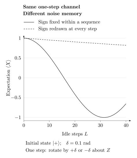
Both models apply $+\delta$ or $-\delta$ with equal probabilities in one step. They differ only in whether that sign persists. Here $\delta=0.1$ rad and the initial state is $|+\rangle$. Negative $\langle X\rangle$ means that the probability of the $X=-1$ outcome exceeds one half; it is not a negative probability. An ideal echo cancels the fixed sign, as explored below.

Slow drift can produce a similar discrepancy between calibration and later use. Record acquisition times, interleave reference circuits and compare short with long sequences. Averaging epochs may hide excess uncertainty: if $N$ conditionally independent shots share a random success probability $q$, the number $K$ of successes obeys

$$\operatorname{Var}K =N\bar q(1-\bar q)+N(N-1)\operatorname{Var}q.$$

The second term vanishes only when this shared fluctuation vanishes. Ordinary binomial error bars can therefore be too small. Explicit time dependence, memory and failure of a chosen exponential fit are distinct statements; Markovian and non-Markovian noise and the open-system discussion explain the formal distinctions (Breuer et al.).

Choosing an experiment and a remedy

Experiment	What it helps determine
Rabi, Ramsey, echo and relaxation measurements	rotation calibration and selected decay mechanisms
Process tomography with trusted references, or gate-set tomography	a channel or a self-consistent preparation–gate–measurement model; stationarity and reference assumptions matter
Randomized benchmarking	an ensemble decay with reduced sensitivity to constant SPAM offsets, not automatic workload accuracy
Simultaneous operations and cycle benchmarks	errors in relevant parallel layers and repeated operations
Held-out application circuits	whether the fitted model predicts outputs, leakage and uncertainty at the depths and times actually used

Use circuits excluded from fitting to test predictions, including different depths and simultaneous operations. Device characterization connects these tests; noise simulation explains how to compare models. A benchmark score such as cross entropy needs its own interpretation and does not alone certify closeness of complete distributions.

A deterministic detuning suggests recalibration or refocusing. Leakage may require pulse changes and explicit detection. Time-varying readout may need fresh calibration. Error mitigation can reduce bias in selected estimated observables, while increasing variance or relying on a model; it generally does not restore a protected state. Quantum error correction instead uses redundancy and syndrome measurements to preserve encoded information. Both approaches must be tested with the correlations and failed attempts present in the intended experiment.

Exercises

1. Coherent accumulation

For $\epsilon=10^{-3}$ and $L=100$, compare the unwanted $X$ rotation’s flip probability with $100$ times its one-cycle value. How can ideal $Z$ pulses cancel two equal rotations?

Solution

$\sin^2(0.05)\simeq0.002498$, whereas $100\sin^2(0.0005)\simeq0.000025$. The angles add before squaring. For the cancellation sequence, $ZV_\epsilon ZV_\epsilon=V_\epsilon^\dagger V_\epsilon=I$. The conclusion assumes ideal instantaneous $Z$ pulses and equal errors.

2. Faults versus output errors

For $L=200$ independent $X$ faults with $p=2\times10^{-4}$, compare the probability of at least one fault with the final flip probability on $|0\rangle$.

Solution

$1-(1-p)^{200}\simeq0.03921$, while $[1-(1-2p)^{200}]/2\simeq0.03845$. The difference includes nonzero even numbers of faults that cancel. Both approach $Lp=0.04$ at leading order, but they are not the same event.

3. Infer a pure-dephasing time

In the exponential two-level model, $T_1=80\,\mu\mathrm{s}$ and $T_2=60\,\mu\mathrm{s}$. Find $T_\phi$. Could $T_2=180\,\mu\mathrm{s}$ describe the same model at that $T_1$?

Solution

$T_\phi^{-1}=1/60-1/160=1/96$ in inverse microseconds, so $T_\phi=96\,\mu\mathrm{s}$. The second value exceeds $2T_1=160\,\mu\mathrm{s}$ and would require a negative pure-dephasing rate. Check measurement uncertainties, pulse sequences and the validity of the matched exponential model before assigning such a rate.

4. Leakage hidden by binary readout

The output of a three-level device is $\rho'=0.70|0\rangle\langle0|+0.25|1\rangle\langle1|+0.05|2\rangle\langle2|$. If the computational space is spanned by $|0\rangle,|1\rangle$, find the leakage and the reported bit-one probability when $|2\rangle$ is assigned to bit one. What happens if leaked outcomes are discarded instead?

Solution

The leakage is $0.05$. Misassignment gives bit-one probability $0.30$. Discarding the leaked outcomes accepts with probability $0.95$ and gives conditional bit-one probability $0.25/0.95=5/19$. These are three different quantities; the accepted probability alone omits a physical failure channel.

5. Correlated classical readout

A detector flips both reported bits with probability $q$ and otherwise reports them correctly. Write its assignment matrix in the order $00,01,10,11$. Why do independent one-bit calibration matrices fail?

Solution

$$A=\begin{pmatrix} 1-q&0&0&q\\0&1-q&q&0\\0&q&1-q&0\\q&0&0&1-q \end{pmatrix}.$$

This is a valid joint classical model. Each marginal detector flips with probability $q$, but their product predicts single-bit errors with probability $q(1-q)$ each. Those events never occur in the actual model. At $q=0.1$, input $00$ produces only $00$ and $11$ with probabilities $0.9,0.1$, whereas the product approximation predicts $0.81,0.09,0.09,0.01$.

6. Equal infidelity, different distances

A qubit channel has average infidelity $r=10^{-4}$. Compare the diamond distance if it is a coherent Pauli overrotation or a stochastic Pauli flip.

Solution

For the overrotation, $|\sin(\epsilon/2)|=\sqrt{3r/2}$, so $|\epsilon|\simeq0.024495$ for the small-angle branch and $D_\diamond\simeq0.012247$. For the stochastic flip, $D_\diamond=p=3r/2=0.00015$. Knowing $r$ without the mechanism does not choose between these values.

7. Echo and shared fluctuations

Insert an ideal instantaneous $X$ pulse halfway through an even number $L$ of the random-sign $Z$ rotations above. Start in $|+\rangle$ and measure $X$. Compare the fixed-sign and independently redrawn models. Separately, if $100$ shots share $q=0.4$ or $0.6$ with equal probabilities, find the mean and variance of their success count.

Solution

Because $XZX=-Z$, the fixed-sign propagator is $U_s^{L/2}XU_s^{L/2}=X$. The initial state is an $X$ eigenstate, so the echo restores $\langle X\rangle=1$. Independent symmetric signs are unaffected statistically by reversing the signs in the second half; their expectation remains $(\cos\delta)^L$.

For the counts, $\bar q=0.5$ and $\operatorname{Var}q=0.01$. Thus $\mathbb E K=50$ and $\operatorname{Var}K=25+100\cdot99\cdot0.01=124$, not the binomial value $25$. Redrawing $q$ independently before every shot would instead give that binomial variance.

References

• H.-P. Breuer, E.-M. Laine, J. Piilo, and B. Vacchini, “Colloquium: Non-Markovian dynamics in open quantum systems,” Reviews of Modern Physics 88, 021002 (2016), doi:10.1103/RevModPhys.88.021002.
• R. Kueng, D. M. Long, A. C. Doherty, and S. T. Flammia, “Comparing experiments to the fault-tolerance threshold,” Physical Review Letters 117, 170502 (2016), doi:10.1103/PhysRevLett.117.170502.
• M. A. Nielsen and I. L. Chuang, Quantum Computation and Quantum Information, 10th anniversary edition, Cambridge University Press, 2010, doi:10.1017/CBO9780511976667.
• T. Proctor, K. Rudinger, K. Young, M. Sarovar, and R. Blume-Kohout, “What randomized benchmarking actually measures,” Physical Review Letters 119, 130502 (2017), doi:10.1103/PhysRevLett.119.130502.
• K. Rudinger, T. Proctor, D. Langharst, M. Sarovar, K. Young, and R. Blume-Kohout, “Probing context-dependent errors in quantum processors,” Physical Review X 9, 021045 (2019), doi:10.1103/PhysRevX.9.021045.
• M. Sarovar, T. Proctor, K. Rudinger, K. Young, E. Nielsen, and R. Blume-Kohout, “Detecting crosstalk errors in quantum information processors,” Quantum 4, 321 (2020), doi:10.22331/q-2020-09-11-321.
• C. J. Wood and J. M. Gambetta, “Quantification and characterization of leakage errors,” Physical Review A 97, 032306 (2018), doi:10.1103/PhysRevA.97.032306.