Cycle Benchmarking

Cycle benchmarking measures the error of a scheduled layer of gates, idles, and simultaneous activity. It repeats a target Clifford layer while inserting random Pauli operations, then measures how selected Pauli expectations decay.

The central idea is to keep the layer of interest fixed while making its noise easier to analyze. The resulting fidelity refers to the dressed cycle, including the implemented randomizing operations. A fitted decay can measure a product of several Pauli responses, so converting it into a fidelity requires care.

Required background. Randomized benchmarking explains decay experiments; Pauli channels explains diagonal noise in a Pauli basis. Helpful background. Stabilizer formalism supplies efficient Clifford propagation.

A scheduled layer is the physical object

A controlled-Z gate applied alone and the same gate applied alongside several drives need not have the same error. Timing, spectators, idles, echo pulses, and frame updates affect the implemented channel. Cycle benchmarking includes this parallel context, rather than inferring a layer’s quality by multiplying isolated component fidelities.

The standard protocol uses a Clifford cycle $G$, which maps every Pauli to another Pauli up to sign. The test remains classically trackable without a large random Clifford inversion. It does not directly characterize an arbitrary non-Clifford layer by the same formulas.

Random Pauli operations may be physical pulses, virtual changes of frame, or corrections absorbed into adjacent gates. Their noise and compilation matter. The ideal Pauli twirl describes a fixed error channel conjugated by perfect randomizers; physical implementations need additional assumptions to realize that model (Wallman and Emerson, 2016). The original cycle-benchmarking analysis assumes Markovian noise and gate-independent noise on the randomizing single-qubit cycles (Erhard and colleagues, 2019).

Pauli responses and process fidelity

For $n$ qubits, set $d=2^n$. The effective implementation below includes the randomizing operations. In the tailored-noise model, use the convention

$$\widetilde{\mathcal G}=\mathcal G\circ\Lambda,$$

so $\Lambda=\mathcal G^{-1}\circ\widetilde{\mathcal G}$ is the relative error before the ideal cycle. Define its response to a Pauli $P$ by

$$f_P=\frac1d\operatorname{Tr}[P\Lambda(P)].$$

For a Pauli channel, $\Lambda(P)=f_PP$. A response near one preserves that Pauli expectation; a smaller response attenuates it.

The process fidelity, or entanglement fidelity relative to $G$, is

$$F_{\rm e}=\frac1{d^2}\sum_P f_P.$$

This Pauli-average identity also holds for a general channel; diagonalization is needed for the simple repeated-cycle decay, not for the identity itself (Flammia and Liu, 2011). Trace preservation gives $f_I=1$, even when the channel is not unital.

If a Pauli channel applies error $Q$ with probability $\mu_Q$, then

$$\begin{aligned} f_P&=\sum_Q\mu_Q\chi(P,Q),\\ \mu_Q&=\frac1{d^2}\sum_P\chi(P,Q)f_P, \end{aligned}$$

where $\chi(P,Q)$ is $+1$ for commuting Paulis and $-1$ otherwise. In particular, $F_{\rm e}=\mu_I$: process infidelity is the nonidentity error probability in this effective Pauli model.

Average gate fidelity uses a different normalization:

$$F_{\rm avg}=\frac{dF_{\rm e}+1}{d+1}.$$

Thus average infidelity is $d/(d+1)$ times process infidelity (Nielsen, 2002). This conversion does not turn a bound or an approximate estimate into an exact fidelity.

Why a controlled-Z experiment measures a product

Ignore known signs temporarily and write the Clifford permutation as $\pi$:

$$\mathcal G(P)=s_P\pi(P), \qquad s_P=\pm1.$$

Under stationary Pauli-diagonal noise, each step attenuates the current Pauli and then moves it to the next one. After correcting the known ideal signs, the selected signal has the form

$$S_P(m)=A_P\prod_{j=0}^{m-1}f_{\pi^j(P)}.$$

The constant $A_P$ represents preparation, readout, and edge effects after the protocol isolates the chosen Pauli component.

For controlled-Z,

$$XI\longmapsto XZ\longmapsto XI.$$

At even lengths, the measured Pauli returns to its initial form:

$$S_{XI}(2t)=A_{XI}(f_{XI}f_{XZ})^t.$$

Writing this as $A_{XI}g^{2t}$ identifies

$$g=\sqrt{f_{XI}f_{XZ}},$$

assuming positive responses. It does not determine the two factors individually.

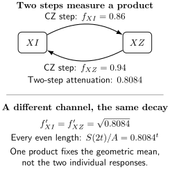
Two applications return the Pauli to its starting point and measure the product $0.86\times0.94=0.8084$. Replacing both factors by $\sqrt{0.8084}\simeq0.899111$ leaves every even-length decay unchanged. The individual responses have different arithmetic means.

More generally, an orbit $\mathcal O$ of length $\ell$ gives

$$g_{\mathcal O}=\left(\prod_{P\in\mathcal O}f_P\right)^{1/\ell}.$$

Use lengths that return to the same ideal measurement procedure. Choosing multiples of the order of the Clifford channel is sufficient. Orbit-compatible lengths can also work when their output signs and measurement amplitudes are controlled.

Turning random measurements into a signal

A practical experiment samples test Paulis, prepares suitable product-basis states, repeats the target with independent Pauli randomizers, and measures the predicted output Pauli. Stabilizer propagation supplies the ideal sign for every circuit. Multiply each recorded outcome by that sign before averaging.

For example, prepare $Z=+1$ and apply one uniformly random Pauli to an otherwise perfect qubit. The raw $Z$ outcomes average to zero: $I,Z$ preserve the sign while $X,Y$ reverse it. Correcting the known sign makes every ideal result $+1$. Forgetting this step would mistake intentional randomization for noise.

The input and measurement randomization must also isolate the desired Pauli component. One useful ideal description uses the mixed eigenstates

$$\rho_\pm=\frac{I\pm P}{d}.$$

They can be prepared as mixtures of product-basis eigenstates. Taking half the difference of their output Pauli expectations isolates the response to $P$ and cancels a constant additive readout offset. Implemented preparation and readout errors still require the protocol’s stability and sign-projection assumptions; an arbitrary raw expectation is not guaranteed to be a single exponential.

At two compatible lengths with the same nonzero amplitude,

$$g_P= \left[\frac{S_P(m_2)}{S_P(m_1)}\right]^{1/(m_2-m_1)}.$$

For $m_1=4$, $m_2=12$, $S(4)=0.842$, and $S(12)=0.790$, the estimate is approximately $0.992063$. The ratio cancels a constant amplitude, not drift between the two measurements. A small denominator makes it unstable; noisy negative or zero signals should be handled by an appropriate likelihood rather than clipped before taking roots.

Use more than two lengths to test the assumed decay. Two points alone cannot reveal an additional mode, changing amplitude, or offset.

The aggregate is a lower bound in the positive-response model

Suppose the experiment samples individual nonidentity Paulis uniformly and assigns each its orbit rate $g_P$. Define the population aggregate

$$F_{\rm CB}=\frac{1+\sum_{P\neq I}g_P}{d^2}.$$

For each orbit, the arithmetic–geometric mean inequality gives

$$g_{\mathcal O}\leq \frac1{|\mathcal O|}\sum_{P\in\mathcal O}f_P.$$

Summing over Paulis, with each orbit weighted by its size, proves

$$F_{\rm CB}\leq F_{\rm e}.$$

This derivation assumes nonnegative responses and the stationary effective Pauli model. It is not a bound for arbitrary fitted decay curves. Negative responses can be hidden by even-length sampling, as Exercise 8 shows.

When $f_P=1-\epsilon_P$ and all errors are small, the orbit’s arithmetic mean exceeds its geometric mean by

$$\frac12\operatorname{Var}_{\mathcal O}(\epsilon_P) +O(\epsilon^3).$$

The discrepancy begins at second order. This explains the accurate lower-bound interpretation in the regime of the original protocol. Equality holds when responses are constant within each orbit.

For instance, consider a physical two-qubit Pauli channel with $f_I=1$, all nonidentity responses $0.9$ except $f_{XI}=0.86$ and $f_{XZ}=0.94$. The inverse Pauli transform gives nonnegative error probabilities. Then

$$\begin{aligned} F_{\rm e}&=0.906250,\\ F_{\rm CB}&\simeq0.906139. \end{aligned}$$

A second physical channel replacing those two responses by their geometric mean has exactly the same controlled-Z orbit decays, but its true process fidelity equals $0.906139$. Thus the missing distinction is real, not merely uncertainty in the fit.

With finite data, replace the Pauli average by its sample mean and estimate each rate from repeated circuits. The resulting point estimate can fluctuate above the population bound and is generally biased by nonlinear ratios and roots. A confidence statement must account for these effects; the population inequality alone does not make every measured value a certified lower limit.

As a numerical conversion, a two-qubit population mean $\overline g_{\neq I}=0.990$ gives

$$F_{\rm CB}=\frac{1+15(0.990)}{16}=0.990625.$$

Under the model this bounds the true average infidelity by $r\leq0.0075$. Calling $0.0075$ the exact average infidelity would discard the orbit ambiguity.

What can and cannot be learned

Information	What the standard decay supplies
A Pauli fixed by the cycle	Its individual positive response
A nontrivial orbit	A product or geometric mean
Uniformly sampled Pauli directions	An aggregate fidelity bound
A complete Pauli error distribution	Additional information is needed

For controlled-Z, $ZI$, $IZ$, and $ZZ$ are fixed. The other twelve nonidentity Paulis form six two-element orbits. Sampling each orbit equally would overweight the fixed directions; sample Paulis uniformly or apply the correct orbit-size weights.

Related cycles and trusted operations can reveal more combinations. In the model studied by Chen and colleagues (2023), Clifford layers have Pauli noise, SPAM is uncertain, and single-qubit controls are ideal or absorbed into a suitable dressed-noise description. A graph of Pauli support patterns characterizes the identifiable products. Its cycles represent products that survive the SPAM ambiguity. This result does not say that one fixed target cycle reveals every response, or that arbitrary noisy controls satisfy the same assumptions.

The total dressed fidelity includes randomizer errors. Dividing it by a reference fidelity does not generally remove those errors. Even independent stochastic Pauli errors can cancel: two bit-flip channels with flip probability $0.1$ each have process fidelity $0.9$, but their composition has fidelity $0.82$, not $0.81$. The ratio $0.82/0.9$ therefore overestimates the second channel’s $0.9$ fidelity.

Statistical cost and limits of the model

There are three sampling questions: which test Paulis were selected, which random circuits were drawn for each Pauli and length, and which outcomes appeared on repeated shots. More shots of existing circuits cannot remove uncertainty from the first two choices. Randomized benchmarking derives the circuit/shot variance and switching-cost tradeoff.

If the exact orbit rates lie in $[0,1]$, $K$ independent uniformly sampled Paulis estimate their mean within $\varepsilon$ with failure probability at most $\delta$ when

$$K\geq\frac{\log(2/\delta)}{2\varepsilon^2}.$$

This elementary bound does not depend on the register dimension. It assumes access to the exact rates: finite-shot rate estimation, small preparation/readout contrast, and small decays add costs. Estimating all $4^n$ responses or rare error probabilities is a much larger task.

Compare several compatible length pairs, interleave their acquisition times, and check computational-space population. Leakage, drift, memory, and randomizer-dependent noise can spoil the stationary Pauli model. For an undressed workload, coherent accumulation can also differ from the averaged randomized experiment. These are physical limits of the inference, rather than problems cured by collecting more shots.

Exercises

1. Recover a Pauli error distribution

A qubit has $f_X=0.98$, $f_Y=0.97$, and $f_Z=0.99$. Find all four error probabilities and both fidelity conventions.

Solution

The inverse transform gives

$$\begin{aligned} \mu_I&=(1+f_X+f_Y+f_Z)/4=0.985,\\ \mu_X&=(1+f_X-f_Y-f_Z)/4=0.005,\\ \mu_Y&=(1-f_X+f_Y-f_Z)/4=0,\\ \mu_Z&=(1-f_X-f_Y+f_Z)/4=0.010. \end{aligned}$$

They are nonnegative and sum to one. Process fidelity is $0.985$ and average fidelity is $(2\times0.985+1)/3=0.990$.

2. Check the controlled-Z orbit

Verify $XI\mapsto XZ\mapsto XI$. If a fitted positive rate is $g=0.991$, what is determined?

Solution

Controlled-Z maps $X_1$ to $X_1Z_2$ and preserves $Z_2$. Applying it twice restores $X_1$. The measured product is $f_{XI}f_{XZ}=0.991^2=0.982081$. One product does not fix both factors.

3. Arithmetic versus geometric means

For the figure’s two responses, calculate the aggregate fidelity gap. Why is the proposed two-qubit channel physical?

Solution

The orbit arithmetic mean is $0.9$, while $g=\sqrt{0.8084}\simeq0.899110672$. Only two of the sixteen Pauli terms differ, so

$$F_{\rm e}-F_{\rm CB}=\frac{2(0.9-g)}{16} \simeq0.000111166.$$

Before the perturbation, $\mu_I=0.90625$ and every other error probability is $0.00625$. The changes $-0.04$ and $+0.04$ in two Pauli responses alter any nonidentity probability by at most $0.08/16=0.005$. All remain nonnegative, and the identity probability is unchanged. The equal-response alternative also remains physical.

4. A changing amplitude

If $S(m_i)=A_i g^{m_i}$, derive the two-length estimate. Use $g=0.99$, $A_2/A_1=0.98$, and $m_2-m_1=8$.

Solution

$$\begin{aligned} \widehat g&=g(A_2/A_1)^{1/8}\\ &=0.99(0.98)^{1/8}\\ &\simeq0.987503. \end{aligned}$$

A two-percent amplitude change makes the apparent per-cycle decay stronger. More shots cannot distinguish this systematic change from a different $g$ using only those two conditions.

5. Random signs and readout offsets

A perfect qubit prepared in $Z=+1$ receives a uniformly random Pauli. Explain the raw and corrected means. Separately, if a readout reports $b+a\langle P\rangle$, what does pairing the two input signs accomplish?

Solution

The raw means are $+1$ for randomizers $I,Z$ and $-1$ for $X,Y$, so the uniform mean is zero. Multiplication by the known ideal sign makes every corrected result $+1$.

For ideal paired inputs with output expectations $\pm f$, the reported values are $b\pm af$. Half their difference is $af$: the offset cancels, while the contrast $a$ remains. Stable contrast can cancel in a length ratio; drifting contrast does not.

6. Fidelity is not multiplicative

Compose two independent bit-flip channels with probabilities $q_1=q_2=0.1$. Find the total no-error probability and explain the failure of a fidelity ratio.

Solution

Two flips cancel. Thus

$$F_{\rm e}^{\rm total} =(1-q_1)(1-q_2)+q_1q_2=0.82.$$

Each channel has fidelity $0.9$, but $0.82/0.9\simeq0.911111$ is not the other’s fidelity. Independence of errors does not make their process fidelities multiplicative.

7. Pauli sampling versus measurement cost

For $\varepsilon=0.01$ and $\delta=0.05$, evaluate the stated bound on sampled Pauli directions. Does it bound the total number of experimental shots?

Solution

$$K\geq\frac{\log40}{2(0.01)^2} \simeq18444.4,$$

so $K=18{,}445$ suffices for the bounded-variable sampling statement. This deliberately conservative result treats orbit rates as known. Measuring each rate with finite precision adds circuit and shot costs; it does not guarantee an experiment of only 18,445 shots.

8. Why the positive-response assumption matters

Take an ideal identity cycle whose implementation applies $Z$ deterministically. What would even-length measurements of $X,Y,Z$ show? What is the true process fidelity?

Solution

The responses are $f_X=f_Y=-1$ and $f_Z=1$. All even powers are one, so sampling only even lengths would resemble a perfect cycle if positive roots were silently imposed. Yet

$$F_{\rm e}=(1-1-1+1)/4=0.$$

The near-identity, positive-response regime is essential for the geometric-mean interpretation. Odd lengths expose the sign reversal in this example.

9. When a mean does not define a physical channel

Can the three numbers $f_X=1$, $f_Y=1$, $f_Z=0.8$ describe a qubit Pauli channel?

Solution

No. Although every response lies in $[-1,1]$, the inverse transform gives

$$\mu_Z=(1-f_X-f_Y+f_Z)/4=-0.05.$$

Complete positivity constrains the responses jointly. Bounding each fitted number separately does not ensure a physical reconstructed channel.

References

• Chen, S., Y. Liu, M. Otten, A. Seif, B. Fefferman, and L. Jiang. “The learnability of Pauli noise.” Nature Communications 14, 52 (2023). arXiv:2206.06362.
• Erhard, A., and colleagues. “Characterizing large-scale quantum computers via cycle benchmarking.” Nature Communications 10, 5347 (2019). doi:10.1038/s41467-019-13068-7.
• Flammia, S. T., and Y.-K. Liu. “Direct fidelity estimation from few Pauli measurements.” Physical Review Letters 106, 230501 (2011). arXiv:1104.4695.
• Nielsen, M. A. “A simple formula for the average gate fidelity of a quantum dynamical operation.” Physics Letters A 303, 249–252 (2002). arXiv:quant-ph/0205035.
• Wallman, J. J., and J. Emerson. “Noise tailoring for scalable quantum computation via randomized compiling.” Physical Review A 94, 052325 (2016). arXiv:1512.01098.