Why Benchmarking Is Hard

A quantum-computer benchmark measures performance on a specified set of tasks under specified conditions. Its result is useful when those tasks resemble the question we want to answer. A good gate score does not by itself predict an algorithm’s accuracy, and a good conditional success rate does not tell us how long an accepted result takes.

The main difficulty is connecting a measured number to a claim about future behavior. This page develops that connection through examples of task selection, coherent errors, sampling, drift, and verification.

Helpful background. Metrics for Quantum Hardware defines fidelity and performance quantities; Noise in Quantum Information distinguishes error mechanisms, and the Circuit Model describes the operations being tested.

Performance depends on the task

Suppose two processors have these success probabilities:

Task family	Processor A	Processor B
Short local circuits	0.99	0.94
Long circuits with distant interactions	0.60	0.85

A benchmark consisting mostly of the first family favors A; one emphasizing the second favors B. Neither ranking is a universal property of the devices.

Let $C$ denote a task, $\lambda$ its implementation choices, and $t$ the operating time. If $q(C,\lambda,t)$ measures output quality, the benchmark average is

$$\overline q= \mathbb E_{C\sim\mu}[q(C,\lambda,t)].$$

The distribution $\mu$ specifies which tasks count and how often. Changing it changes the question. The same applies to changing the qubit subset, compiler, required accuracy, or allowed mitigation.

Blume-Kohout and Young’s volumetric framework makes this dependence visible by testing circuit width and depth separately. A width–depth performance plot can reveal a preference for narrow deep circuits or wide shallow ones that a single score hides. An application still needs tests of its own structure.

Interpret the scale too. A score $2^{m_*}$ doubles when the largest passing integer size $m_*$ increases by one. This is how a quantum-volume score is constructed; it does not imply that applications run twice as fast. See Quantum Volume and Application Benchmarks and the protocol of Cross and colleagues.

Measurements combine preparation, operations, and readout

For a prepared state $\rho$, implemented circuit $\mathcal C$, and measurement effect $M_x$, the observed probability is

$$p(x)=\operatorname{Tr}[M_x\mathcal C(\rho)].$$

A discrepancy can come from any of these ingredients. Even a single observed flip rate does not generally identify its cause. For independent binary flips during preparation and readout, with probabilities $a$ and $b$,

$$p_{\rm flip}=a(1-b)+(1-a)b.$$

Preparation error $a=0.02$ with perfect readout and perfect preparation with readout error $b=0.02$ give the same observed rate. More repetitions of that one experiment cannot distinguish them. Additional trusted operations, measurement settings, or model assumptions are needed.

State Tomography reconstructs a state under a measurement model; Process Tomography also depends on preparation assumptions. Joint estimation has its own identifiability and gauge issues.

Standard Clifford Randomized Benchmarking uses random sequences and their inverse. With stationary, gate-independent Markovian errors, its sequence-averaged survival has the form

$$P(m)=A p^m+B.$$

Preparation and measurement affect the coefficients $A,B$ in this model, while the decay parameter has a separate interpretation. This does not make every preparation or measurement error harmless, particularly when it depends on sequence length or time. Magesan, Gambetta, and Emerson develop the model and controlled departures from it. A plausible exponential fit alone does not establish all its assumptions.

Equal gate infidelity can hide different circuit errors

Consider an intended identity operation on one qubit. Compare a fixed coherent rotation

$$U_\epsilon=e^{-i\epsilon Z/2}$$

with an independent phase-flip channel at each step,

$$\mathcal D_p(\rho)=(1-p)\rho+pZ\rho Z.$$

Use the same average gate infidelity for both:

$$p=\sin^2(\epsilon/2),\qquad r_1=\frac{1-\cos\epsilon}{3}.$$

Here $r=1-F_{\rm avg}$ averages the input-state fidelity over uniformly distributed pure qubit states. It is not a probability that a gate suffers an independently detectable failure. For the unitary, the identity $F_{\rm avg}=(|\operatorname{Tr}U|^2+2)/6$ gives the expression above. For the phase-flip channel, $r_1=2p/3$.

After $L$ identical coherent steps, the rotation angle is $L\epsilon$. For independent phase flips, the transverse Bloch components acquire a factor $(1-2p)^L=(\cos\epsilon)^L$. Therefore

$$\begin{aligned} r_L^{\rm coh}&=\frac{1-\cos(L\epsilon)}{3},\\ r_L^{\rm stoch}&=\frac{1-(\cos\epsilon)^L}{3}. \end{aligned}$$

For small $\epsilon$ and sufficiently short sequences,

$$r_L^{\rm coh}\approx L^2r_1,\qquad r_L^{\rm stoch}\approx Lr_1.$$

The first approximation requires $|L\epsilon|\ll1$; the second requires $L\epsilon^2\ll1$. Outside these limits use the exact expressions. Coherent infidelity can oscillate rather than grow forever.

For $\epsilon=0.02$ radians, both single-step infidelities are approximately $6.67\times10^{-5}$. After 100 steps, they become approximately $0.472$ and $0.00660$ respectively.

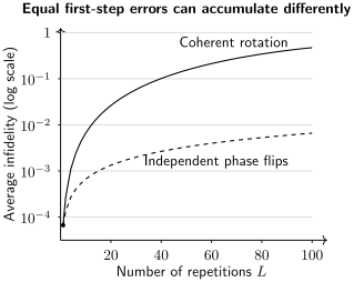
Both errors have the same single-step average infidelity at $\epsilon=0.02$ radians. The solid curve adds rotation angles coherently; the dashed curve represents independent phase flips. These exact curves describe repeated identity targets, not arbitrary circuits.

The example does not say every coherent error accumulates quadratically in every algorithm. Intervening gates can rotate, reinforce, or cancel it. Simultaneous operations, spectator states, leakage, and environmental memory can add further dependence on context. Rudinger and colleagues study tests that detect such changes. Cycle Benchmarking examines operation layers; application tests probe other relevant contexts.

More shots and more circuits answer different questions

Suppose $M$ circuits are drawn independently from the target population. Circuit $i$ succeeds with probability $p_i$ and is repeated $N$ times. Assume shots are independent conditional on that circuit, circuits are independent, and the device is stable. The average of their success frequencies estimates $\mu=\mathbb E_C[p_C]$.

Let $\tau^2=\operatorname{Var}_C(p_C)$. Conditioning first on the circuits and then averaging gives

$$\operatorname{Var}(\widehat\mu) =\frac{\tau^2}{M} +\frac{\mathbb E_C[p_C(1-p_C)]}{MN}.$$

The first term is uncertainty from sampling circuits; the second comes from repeated measurements on each sampled circuit. Increasing $N$ reduces only the second term.

For a population with equal numbers of circuits having $p_C=0.1$ and $p_C=0.9$, the mean is $0.5$, $\tau^2=0.16$, and $\mathbb E[p_C(1-p_C)]=0.09$. With the same budget of 2,000 shots:

Number of circuits M	Shots per circuit N	Standard deviation of estimated population mean
20	100	0.0897
200	10	0.0291
2,000	1	0.0112

The last row assumes drawing and setting up a new circuit has no additional cost. With setup costs or a need to estimate each circuit separately, the best allocation changes. Wallman and Flammia analyze sequence sampling and confidence in randomized benchmarking.

If the goal is instead the average over a fixed, prescribed list of circuits, the list is not a random sample for that claim. Its shot uncertainty is a conditional quantity. Specify whether a result concerns that list or a larger population. Pooling all shots into an independent binomial model can otherwise understate uncertainty substantially.

Time variation changes the model

Suppose a survival factor is $p_1$ for half the experiment and $p_2$ for the other half, with equal weighting at each sequence length. Ignoring common amplitude and offset terms, the averaged signal is

$$\overline f(m)=\frac{p_1^m+p_2^m}{2}.$$

It is generally different from $((p_1+p_2)/2)^m$. For $p_1=0.8$ and $p_2=1$, the length-two values are $0.82$ and $0.81$. Thus fitting the averaged data need not return the average physical parameter. If different lengths are measured in different time windows, even the mixing weights can depend on length.

Retain acquisition times, interleave task families, and repeat reference circuits throughout a run. This helps distinguish task dependence from drift; it does not guarantee stationarity. Proctor and colleagues develop time-resolved detection and tracking. Calibration Loops explains how such changes affect control.

Selection is another source of optimism. Choosing the best qubit subset, compiler seed, or fit range after viewing results uses the data for tuning. Confirm the chosen method on independent evaluation data and include the search cost. Repeated-testing calculations appear in Reproducible Notebooks.

Compare implementations at the same output requirement

A source circuit and a physical experiment are different objects. Routing, native gates, pulse schedules, reset, and classical feedback can change the work performed. Mills and colleagues demonstrate why compilation belongs in comparisons of complete computing systems.

There are two useful questions. Which complete system solves this task best? Allow the declared optimization budget and compare final output quality and total cost. What causes a particular difference? Change one factor at a time within a controlled experiment and measure the response.

Using one compiler version or disabling optimization does not automatically isolate hardware. Different native gates, connectivity, calibration inputs, and schedules can still change the physical workload. A controlled comparison must identify which of these are fixed or varied.

Postselection also changes the cost. If a method accepts a fraction $a$ and has conditional correctness $c$, then

$$P(\text{accepted and correct})=ac.$$

For $a=0.04$ and $c=0.995$, this is $0.0398$ per raw attempt. Independent trials require on average $1/a=25$ attempts to obtain an accepted outcome. That outcome is correct with probability $c$; acceptance alone does not certify correctness.

Compare elapsed time at matched accuracy and confidence, with compilation, preparation, raw shots, optimization, retries, and postprocessing included as appropriate to the question. A latency benchmark and a throughput benchmark can legitimately favor different systems. A comparison with a classical method should identify the algorithm, approximation, software, hardware, input access, and timing boundary. A later improved baseline can change the comparison without changing the original measurement.

A feasible check may leave important errors unseen

An arbitrary $n$-qubit density matrix has $4^n-1$ real parameters. Full reconstruction is expensive; scalable tests therefore often estimate selected properties. Their usefulness depends on which differences they can reveal.

For example, the three-qubit states

$$|\mathrm{GHZ}_\pm\rangle= \frac{|000\rangle\pm|111\rangle}{\sqrt2}$$

are orthogonal but have identical reduced states on every proper subset of qubits. Local checks cannot determine their relative phase. The global observable $X\otimes X\otimes X$ distinguishes them.

A conserved parity, a correct energy, or agreement on a small solvable instance is valuable but does not determine an entire large output state or distribution. Known-answer mirror circuits are useful tests, though their structure may differ from the intended application.

Likewise, a cross-entropy score correlates samples with ideal probabilities; it is not generally a distance from the ideal distribution. Its relation to fidelity requires further assumptions. Cross-Entropy Benchmarking explains these distinctions.

When exact classical calculation is impractical, combine checks that address different possible failures and state what remains unconstrained. Computational hardness is not a test that an experimental output is correct. Verification of Quantum Advantage discusses the stronger requirements for comparative claims.

For a readable account of a benchmark, give the task population, output criterion, implementation choices, sampling design, measured result with uncertainty, and included costs. Link the circuits, counts, and analysis needed to reconstruct the comparison. Reporting Standards develops these details.

Exercises

1. Find the ranking crossover

In the opening table, task family one occurs with probability $w$. When does A have higher mean success?

Solution

$$\begin{aligned} S_A&=0.99w+0.60(1-w),\\ S_B&=0.94w+0.85(1-w). \end{aligned}$$

Their difference is $0.30w-0.25$, so A ranks higher when $w>5/6$. At equality they tie. The task distribution is part of the comparison.

2. Compare two errors with the same single-step score

Take $\epsilon=0.01$ radians and $L=100$. Compute the exact coherent and phase-flip average infidelities, matching their single-step infidelity.

Solution

Both have $r_1\approx1.66665\times10^{-5}$. The repeated values are

$$\begin{aligned} r_{100}^{\rm coh}&=(1-\cos1)/3\\ &\approx0.15323,\\ r_{100}^{\rm stoch}&=(1-(\cos0.01)^{100})/3\\ &\approx0.0016625. \end{aligned}$$

The quadratic coherent approximation gives about $0.16667$, already noticeably inaccurate because $L\epsilon=1$. The linear stochastic approximation remains accurate because $L\epsilon^2=0.01$.

3. Change the sampling allocation

Derive the variance for the 20-circuit, 100-shot design above. Compare it with treating all 2,000 outcomes as independent Bernoulli observations of mean $1/2$.

Solution

$$\begin{aligned} \operatorname{Var}(\widehat\mu) &=0.16/20+0.09/2000\\ &=0.008045. \end{aligned}$$

Its standard deviation is about $0.0897$. The independent-binomial calculation gives variance $0.25/2000=0.000125$ and standard deviation $0.0112$. Shots on one sampled circuit share its success probability, which creates dependence when averaging over the circuit population.

4. Average signals before fitting parameters

For equal populations with decay factors $0.8$ and $1$, find the effective factor inferred from length one alone and from length two alone, assuming a pure exponential with fixed unit amplitude and zero offset.

Solution

Length one gives $p_{\rm eff}=0.9$. Length two gives

$$p_{\rm eff}=\sqrt{0.82}\approx0.90554.$$

They disagree because a mixture of these two exponentials is not one exponential. Adding free fit parameters can conceal some discrepancy over a finite range; a good fit does not prove a stationary physical mechanism.

5. Include rejected attempts

A method accepts 4% of attempts, with conditional correctness 99.5%. What are its accepted-correct probability and mean number of attempts to obtain an accepted outcome under independent repetition?

Solution

They are $0.04(0.995)=0.0398$ and $1/0.04=25$. The mean counts attempts until acceptance. It does not give a stopping rule for correctness unless correctness can also be recognized.

6. Explain a disappearing circuit

A compiler replaces an ideal circuit $UU^\dagger$ by the identity. Does excellent performance on the simplified circuit demonstrate accurate implementation of the gates in $U$?

Solution

No: those gates were not executed. The optimization can be useful if the task is to implement the overall identity efficiently. If the question is how accurately the device executes the original gate sequence, the test must preserve that sequence or otherwise prevent the cancellation. Neither interpretation is meaningful without specifying the task.

7. Find a local-measurement blind spot

Trace out the third qubit of $|\mathrm{GHZ}_+\rangle$ and $|\mathrm{GHZ}_-\rangle$. Then evaluate $X\otimes X\otimes X$.

Solution

Both reduced states are

$$\rho_{12}=\tfrac12 \left(|00\rangle\langle00|+|11\rangle\langle11|\right).$$

The cross terms vanish because $\langle0|1\rangle=0$ on the traced qubit. The global $X$ product exchanges $|000\rangle$ and $|111\rangle$, giving expectation $+1$ and $-1$ respectively.

8. Identify an ambiguous detector model

An experiment prepares the nominal state zero and observes outcome one with probability 0.02. Give two independent preparation/readout flip models that agree with that observation. Can more repetitions choose between them?

Solution

$(a,b)=(0.02,0)$ and $(0,0.02)$ both fit. More repetitions refine the same probability and do not identify its decomposition. Other experiments or trusted calibration information are needed.

9. Interpret a tradeoff

At the same output accuracy, A needs 10 seconds and 100,000 shots; B needs 25 seconds and 20,000 shots. Does either dominate on these two costs?

Solution

No. A uses less time and B fewer shots. Both are undominated among these candidates. A preferred choice needs an additional objective or constraint. Neither the shot count nor the latency alone determines energy cost.

10. Test whether a score is a distance

For two outcomes, let the ideal distribution be $p=(3/4,1/4)$. Define the unnormalized linear cross-entropy score

$$S(q)=2\sum_xq(x)p(x)-1.$$

Compare $q=p$ with the sampler $q=(1,0)$.

Solution

$$\begin{aligned} S(p)&=2(9/16+1/16)-1=1/4,\\ S((1,0))&=2(3/4)-1=1/2. \end{aligned}$$

The sampler that always returns the most likely output has a higher score, although its total variation distance from $p$ is $1/4$ instead of zero. This is a simple counterexample to treating this score as distributional closeness. Practical XEB protocols specify their circuit ensemble and normalization; converting a score into fidelity adds model assumptions.

References

• R. Blume-Kohout and K. C. Young, “A volumetric framework for quantum computer benchmarks,” Quantum 4, 362 (2020), doi:10.22331/q-2020-11-15-362 — task-dependent width–depth comparisons.
• A. W. Cross, L. S. Bishop, S. Sheldon, P. D. Nation, and J. M. Gambetta, “Validating quantum computers using randomized model circuits,” Physical Review A 100, 032328 (2019), doi:10.1103/PhysRevA.100.032328 — quantum-volume protocol and score.
• E. Magesan, J. M. Gambetta, and J. Emerson, “Scalable and robust randomized benchmarking of quantum processes,” Physical Review Letters 106, 180504 (2011), doi:10.1103/PhysRevLett.106.180504 — decay models and their assumptions.
• D. Mills, S. Sivarajah, T. L. Scholten, and R. Duncan, “Application-motivated, holistic benchmarking of a full quantum computing stack,” Quantum 5, 415 (2021), doi:10.22331/q-2021-03-22-415 — compilation and application-motivated comparisons.
• T. Proctor et al., “Detecting and tracking drift in quantum information processors,” Nature Communications 11, 5396 (2020), doi:10.1038/s41467-020-19074-4 — time-resolved characterization.
• K. Rudinger, T. Proctor, D. Langharst, M. Sarovar, K. Young, and R. Blume-Kohout, “Probing context-dependent errors in quantum processors,” Physical Review X 9, 021045 (2019), doi:10.1103/PhysRevX.9.021045 — dependence on operating context.
• J. J. Wallman and S. T. Flammia, “Randomized benchmarking with confidence,” New Journal of Physics 16, 103032 (2014), doi:10.1088/1367-2630/16/10/103032 — sequence sampling and statistical confidence.