Algorithmic Benchmarking

Algorithmic benchmarking asks how accurately, reliably and quickly an implementation solves a specified task. The measured object includes the work needed to turn the input into an accepted answer: preparation, quantum execution, classical processing, measurement, and any necessary retries.

A short circuit at excellent parameters may perform well even when finding those parameters is expensive. Conversely, a noisy circuit may still solve a tolerant task reliably. The benchmark should begin with the answer the user needs, then measure its cost. Proctor and colleagues (2025) place these algorithm-level questions within the broader range of quantum-computer benchmarks.

Required background. Application benchmarks explains task-specific scores and timing boundaries; algorithmic primitives explains coherent input access and readout. Helpful background. The quantum software stack identifies the classical and quantum stages of execution.

The task and its accepted answer

For an input instance $I$, define an output loss $L(I,y)$ and tolerance $\epsilon$. The acceptable answers form

$$\mathcal Y_\epsilon(I)=\{y:L(I,y)\leq\epsilon\}.$$

An algorithm returns a random output $\widehat y$, with success probability

$$p_I=\Pr[\widehat y\in\mathcal Y_\epsilon(I)].$$

Success might mean producing a factor that passes integer multiplication, estimating an energy to a stated accuracy, or finding a feasible solution above a target objective. Sampling an entire distribution is a different task from producing one valid answer. A reference state overlap or gate fidelity can help diagnose an implementation, but does not replace the chosen output criterion.

Three useful experimental boundaries are:

Test	Included computation	Example
Kernel	A specified subroutine with supplied inputs	Evaluate energy at fixed parameters
Algorithm execution	Preparation, iteration and decoding	Run a variational optimizer
Complete solution	Input processing through accepted answer	Include validation, failures and retries

These are useful distinctions, not grades of scientific merit. A kernel test can isolate a fault. It should not be described as the cost of solving a problem whose difficult preprocessing was supplied for free.

Fix the acceptance rule before inspecting results. If success cannot be recognized directly, include a verifier with stated errors, or describe the output quality as estimated. A claim of “repeat until correct” needs a way to identify correctness.

Repeated attempts and time to success

First consider one fixed instance. Suppose independent attempts succeed with constant probability $0<p<1$ and each takes time $t$. The probability of no success in $R$ attempts is $(1-p)^R$. To reach success probability at least $\gamma$,

$$R_\gamma= \left\lceil\frac{\ln(1-\gamma)}{\ln(1-p)}\right\rceil.$$

The fixed-budget time is $R_\gamma t$. The expected time when stopping at the first recognizable success is instead

$$\mathbb E[T]=\frac{t}{p}.$$

These answer different questions: a mean waiting time is not a high-confidence budget. For $p=0.25$ and $t=20$ s, the mean is 80 s, whereas a 95% success budget requires 11 attempts and 220 s. If $p=1$, one attempt suffices; if $p=0$, no finite repetition budget succeeds. Time-to-solution comparisons of randomized solvers are discussed by Rønnow and colleagues (2014).

Successful runs can take longer

Allow the duration $t_r$ and success indicator $Z_r$ of an attempt to be correlated. Assume the pairs $(t_r,Z_r)$ are independent and identically distributed across attempts, with finite mean duration and success probability $p>0$. A renewal argument gives

$$\mathbb E[T]=\mathbb E[t]+(1-p)\mathbb E[T],$$

so the exact mean remains

$$\mathbb E[T]=\frac{\mathbb E[t]}{p}.$$

Independence of duration and success within an attempt is unnecessary. The average duration must include both outcomes. Equivalently,

$$\mathbb E[T] =\frac{1-p}{p}\mathbb E[t\mid Z=0] +\mathbb E[t\mid Z=1].$$

If failures take 20 s, successes 40 s, and $p=0.25$, the mean is $3(20)+40=100$ s. The unconditional attempt mean is 25 s, giving the same $25/0.25=100$ s.

Drift, adaptive restarts, accumulated optimizer state and a changing stopping policy can break the identical-independent-attempt assumption. A one-time setup cost is added once, not multiplied by the expected retries. Variable durations also mean that $R_\gamma\mathbb E[t]$ is not automatically a deadline guaranteeing success probability $\gamma$; a deadline requires the joint distribution of durations and outcomes.

Average over instances after calculating their costs

Now draw an instance $I$ from a specified population and keep retrying that same instance. Its success probability $p_I$ may differ greatly from another’s. The population mean solution time is

$$\mathbb E_I\left[\frac{\mathbb E[t\mid I]}{p_I}\right].$$

It generally differs from dividing the mean attempt time by the mean success probability.

For equally frequent easy and hard instances with $p_I=0.9$ and $0.1$, and one-second attempts,

$$\mathbb E_I\mathbb E[T\mid I] =\frac12\left(\frac1{0.9}+\frac1{0.1}\right) \simeq5.56\ \mathrm s.$$

Using the pooled success probability $0.5$ would predict only 2 s. That describes a different experiment in which a fresh independent instance is drawn on every attempt and solving any one is sufficient.

The same distinction changes finite-budget failure probabilities:

$$\begin{aligned} P_{\rm fixed}(R)&=\tfrac12(0.1^R+0.9^R),\\ P_{\rm fresh}(R)&=0.5^R. \end{aligned}$$

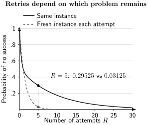
The same average single-attempt success probability can hide different retry behavior. After five attempts, the fixed-instance mixture still fails with probability $0.29525$; replacing it by a fresh instance on every attempt gives $0.03125$. Both curves use equal initial weights and success probabilities $0.9$ and $0.1$.

For the fixed-instance experiment, failures increasingly concentrate on the hard cases. Report per-instance results or relevant quantiles, including unsolved and timed-out cases. A timeout tells us that the completion time exceeds the cutoff; it is not a completed solution with that runtime. If any positive-weight instances have $p_I=0$, the unrestricted mean time to solve the population is infinite.

Input access and state preparation cost

A quantum query is an operation supplied by an input model. A hardware benchmark must implement it. Explicit arrays, sparse-entry oracles, block encodings and prepared quantum states are different forms of access; give the classical comparator equivalent information and count relevant preprocessing.

For one uniformly located marked item among $N$ candidates, the leading ideal search costs are approximately

$$\begin{aligned} C_Q&\simeq\frac\pi4c_Q\sqrt N,\\ C_C&\simeq\frac12c_CN. \end{aligned}$$

Here $c_Q$ is the cost of a coherent predicate call and $c_C$ a classical predicate evaluation. The classical expression describes searching without replacement until the marked item is found. Ignoring preparation, reflections and verification, the leading crossover is

$$N_\times\simeq \left(\frac{\pi c_Q}{2c_C}\right)^2.$$

This is an illustrative cost model, not a measured advantage. Grover search gives the actual success law and query count. Babbush and colleagues (2021) discuss how fault-tolerant overhead can offset a quadratic asymptotic improvement.

State preparation introduces another success factor. If the desired eigenspace has projector $\Pi_\star$, the input’s weight is

$$a=\langle\psi_0|\Pi_\star|\psi_0\rangle.$$

In ideal phase estimation, that sector is sampled with probability $a$. If the conditional probability of a sufficiently accurate readout is $b$, the desired event has probability $ab$, provided false acceptance from other sectors is excluded. This is a conditional chain rule; it does not assume that unrelated marginal success probabilities multiply. Small overlap can dominate the retry cost even when each phase estimate is precise.

Output access matters too. Preparing a state encoding a solution vector does not print all its entries. If the task needs a classical vector, count its extraction to the required accuracy. Dalzell and colleagues (2023) analyze how input conditioning, constant factors and output tomography affect an end-to-end quantum optimization resource estimate.

Hybrid optimization must include its search

A variational eigensolver estimates

$$E(\theta)=\sum_\alpha h_\alpha \langle P_\alpha\rangle_\theta$$

and changes $\theta$ using classical optimization. Its execution cost includes every tested parameter setting, measurement group, gradient shift, restart and final check. Evaluating only the final circuit omits the search for its parameters. Tilly and colleagues (2022) review these components and their practical costs.

For example, 40 iterations with six measurement circuits per iteration and 500 shots each use 120,000 shots. Adding 10,000 independent final-validation shots gives 130,000. At 100 microseconds per shot that is 13 s of shot execution, before communication and classical processing. If 240 separate submissions each incur 50 ms of serial overhead, they add another 12 s. Batching changes this latency model and should be described.

Selecting the smallest of many noisy energy estimates also favors downward fluctuations. Re-estimate the final parameters with fresh data. This separates parameter selection from assessment; it does not by itself remove systematic measurement bias.

For a physical state $\rho$, a known nondegenerate ground energy $E_0$, and gap $\Delta=E_1-E_0>0$,

$$1-\langle u_0|\rho|u_0\rangle \leq\frac{\operatorname{Tr}(\rho H)-E_0}{\Delta}.$$

Thus energy accuracy implies ground-state fidelity only relative to a known gap. For a degenerate ground space, replace the overlap by its projector weight. A noisy or mitigated energy estimator is not necessarily the exact expectation of a physical state; a value below $E_0$ cannot be inserted into this bound as proof of fidelity greater than one.

Acceptance, precision and useful samples

Postselection retains only a fraction $a$ of raw trials. If independent trials have a fixed acceptance probability and acquisition stops after $M$ accepted samples, the negative-binomial mean is exactly

$$\mathbb E[N_{\rm raw}]=\frac{M}{a}.$$

A fixed budget of $M/a$ trials produces only $M$ accepted samples on average; it does not guarantee obtaining that many. Acceptance uncertainty, drift, and correlation require additional analysis. Rejected trials still consume time, and the retained distribution is conditional on the acceptance event. Error mitigation explains when that conditional estimator answers the original question.

For an estimated observable, separate squared bias and variance:

$$\operatorname{MSE}(\widehat\theta) =\operatorname{Bias}(\widehat\theta)^2 +\operatorname{Var}(\widehat\theta).$$

If an independent reference has a proven absolute error at most $\epsilon_{\rm ref}$ and the estimator is within $\epsilon_{\rm est}$ of that reference, the triangle inequality gives total error at most their sum. Such addition requires comparable error quantities. Do not add a probability of failure, an energy error and a channel infidelity as though they shared units. Failure probabilities can instead be combined by a union bound, without assuming independence.

For correlated samples, effective sample size depends on the observable. With stationary normalized autocorrelation $\rho_O(k)$, use the convention

$$\tau_{{\rm int},O}=\frac12+\sum_{k\geq1}\rho_O(k).$$

When the correlation sum converges and the record is long enough,

$$N_{{\rm eff},O}\simeq\frac{N}{2\tau_{{\rm int},O}}.$$

Independent samples have $\tau_{\rm int}=1/2$, so $N_{\rm eff}=N$. This describes the variance of a sample mean for that observable, not a universal number of independent draws from the entire distribution.

Comparing sizes, implementations and classical methods

Use the same tasks, instance population, output tolerance and success target for both sides. Algorithm and compiler tuning should use separate validation data or a declared shared tuning budget. Equal-instance averaging differs from pooling unequal numbers of repeated runs; choose the weights that answer the intended question.

Problem size alone often hides difficulty. Linear solvers depend on conditioning, state preparation on structure, and spectral algorithms on gaps and precision. Vary those features as well as the size. A result on well-conditioned examples does not establish performance on all matrices.

Keep two scaling experiments distinct. Strong scaling holds a problem fixed while adding computational resources. Weak scaling increases the workload in proportion to resources so the workload per resource stays approximately fixed. A general problem-size sweep is not automatically weak scaling.

A crossover extrapolated from small runs depends on the fitted model, constants, fixed costs and classical implementation. Test plausible alternative models and matched overlap regimes before treating the projection as predictive. Keep resource estimates separate from measured executions, especially for proposed error-corrected algorithms. Verification of quantum advantage addresses the additional classical comparison and correctness claims.

Exercises

1. Mean time and a success budget

For independent 20 s attempts with success probability $0.25$, calculate the mean stopping time and the time budget for at least 95% success.

Solution

The mean is $20/0.25=80$ s. Since $\ln(0.05)/\ln(0.75)\simeq10.413$, the budget is 11 attempts, or 220 s. Ten attempts succeed with probability about $0.9437$; eleven give about $0.9578$.

2. Correlation within each attempt

Successful attempts take 40 s, failures 20 s, and success probability is $0.25$. Independent attempts continue until success. Find the expected time and explain why duration–success correlation does not invalidate the result.

Solution

The expected number of failures is $(1-p)/p=3$, giving $3(20)+40=100$ s. Alternatively, the mean attempt duration is $0.25(40)+0.75(20)=25$ s, so $\mathbb E[t]/p=100$ s. The renewal calculation needs independent identical attempts, not independence of the duration and outcome of the same attempt.

3. Keeping the hard instance

For the equal mixture of success probabilities $0.9$ and $0.1$, calculate the population success probability after five total attempts on the initially chosen instance. Compare it with using the average probability in a geometric model.

Solution

With five total attempts, the failure probability is

$$P_{\rm fixed}(5)=\tfrac12(0.1^5+0.9^5)=0.29525.$$

Success is $0.70475$. The pooled model would predict $1-0.5^5=0.96875$, which applies when a fresh independent instance is drawn each attempt. Repetition does not turn a hard fixed instance into an average one.

4. State overlap and phase estimation

An input has target-sector weight $0.05$ and conditional accurate-readout probability $0.8$. One run takes 2 s. Assuming recognizable successes and independent attempts, find a 95% success budget.

Solution

The success probability is $0.05(0.8)=0.04$. Therefore

$$R_{0.95}=\left\lceil\frac{\ln0.05}{\ln0.96}\right\rceil=74.$$

The budget is 148 s, excluding any one-time setup. The mean time to first success is instead $2/0.04=50$ s.

5. An expensive coherent query

Let $c_Q/c_C=10^4$ in the search comparison. Estimate the leading crossover and identify omitted work.

Solution

Equating the leading costs gives

$$N_\times\simeq\frac{\pi^2}{4}10^8 \simeq2.47\times10^8.$$

Preparation, reflections, error correction, measurement, retries and verification may shift the practical crossover. This calculation concerns the specified predicate costs and ideal search model, not every task with $N$ inputs.

6. Selection can lower a noisy energy

Two independently evaluated parameter settings have the same true energy. Each measured energy error is independently $+\sigma$ or $-\sigma$, equally likely. What is the mean error of the lower reported energy? What does independent reevaluation change?

Solution

Both errors are positive with probability $1/4$; otherwise the minimum is $-\sigma$. The selected mean error is $\sigma/4-3\sigma/4=-\sigma/2$. A fresh unbiased estimate at the chosen setting has zero mean measurement error. It does not make the chosen setting better than its true energy or remove systematic bias.

7. The role of a spectral gap

A physical state’s exact energy exceeds a nondegenerate ground energy by 0.002 in the chosen energy units. What fidelity lower bound follows if the gap is 0.1? What changes if the gap is 0.001?

Solution

The excited-state weight is at most $0.002/0.1=0.02$, so ground-state fidelity is at least $0.98$. With gap $0.001$, the bound would be $F\geq-1$, which supplies no information beyond $F\geq0$. An energy tolerance is meaningful for fidelity only relative to the spectral gap and trustworthy energy uncertainty.

8. Accepted counts are random

Independent raw trials are accepted with probability $0.12$. Compare stopping at 6,000 accepted trials with taking exactly 50,000 raw trials.

Solution

Stopping at 6,000 successes has mean raw count $6000/0.12=50{,}000$ and negative-binomial variance

$$\operatorname{Var}(N_{\rm raw}) =\frac{6000(0.88)}{0.12^2} \simeq366{,}667.$$

For a fixed 50,000-trial budget, the accepted count is binomial with mean 6,000 and standard deviation $\sqrt{50000(0.12)(0.88)}\simeq72.66$. Neither experiment makes both counts deterministic.

9. Reference uncertainty and correlated samples

A measured discrepancy is 0.003 and a proven reference error is at most 0.002. What deterministic error bound follows? Separately, if an observable has $\rho_O(k)=0.8^k$, estimate its effective sample size for $N=9000$.

Solution

The triangle bound is 0.005; it is not a quadrature sum unless a suitable random-error model is supplied. The correlation sum gives

$$\tau_{{\rm int},O}=\frac12+\frac{0.8}{1-0.8}=4.5,$$

so $N_{{\rm eff},O}\simeq9000/9=1000$. This is an asymptotic variance comparison for that observable.

10. A ratio with a negative optimum

A maximization problem has optimum $-2$. Compare feasible outputs $-3$ and $-5$ using the ratio to the optimum and using the optimality gap.

Solution

The ratios are $1.5$ and $2.5$, so treating a larger ratio as better rewards the worse solution. The gaps are $(-2)-(-3)=1$ and $(-2)-(-5)=3$, correctly identifying $-3$ as closer. If the optimum is not known, rigorous bounds on it give bounds on the gap; a best-known value is not automatically the exact optimum.

References

• Babbush, R., J. R. McClean, M. Newman, C. Gidney, S. Boixo, and H. Neven. “Focus beyond quadratic speedups for error-corrected quantum advantage.” PRX Quantum 2, 010103 (2021). arXiv:2011.04149.
• Dalzell, A. M., and colleagues. “End-to-end resource analysis for quantum interior point methods and portfolio optimization.” PRX Quantum 4, 040325 (2023). arXiv:2211.12489.
• Proctor, T., K. Young, A. D. Baczewski, and R. Blume-Kohout. “Benchmarking quantum computers.” Nature Reviews Physics 7, 105–118 (2025). arXiv:2407.08828.
• Rønnow, T. F., and colleagues. “Defining and detecting quantum speedup.” Science 345, 420–424 (2014). arXiv:1401.2910.
• Tilly, J., and colleagues. “The variational quantum eigensolver: a review of methods and best practices.” Physics Reports 986, 1–128 (2022). arXiv:2111.05176.