VQE

The variational quantum eigensolver (VQE) estimates the lowest eigenvalue of a specified Hermitian operator $H$ by minimizing its expectation value over a parameterized family of quantum states:

$$E(\boldsymbol{\theta}) = \langle \psi(\boldsymbol{\theta}) \rvert H \lvert \psi(\boldsymbol{\theta}) \rangle.$$

If $E_0$ is the exact ground-state energy of $H$, the Rayleigh–Ritz principle gives

$$E(\boldsymbol{\theta}) \geq E_0$$

for every normalized trial state. A quantum processor prepares the trial state and estimates terms in $H$; a classical optimizer chooses new parameters. VQE trades the long coherent evolution used by phase estimation for many shorter state preparations, measurements, and adaptive quantum–classical round trips.

The method applies to a supplied finite-dimensional Hamiltonian. Its variational bound refers to that operator and, when imposed, a specified symmetry sector. It does not by itself bound the error of a molecular model relative to experiment, guarantee that an optimizer finds the best trial state, or establish a computational advantage.

Helpful background. The variational principle explains why trial-state energies bound the ground energy; variational quantum algorithms develops parameter optimization and measurement uncertainty. Many-particle Hamiltonians supplies the second-quantized notation used in the chemistry example.

The first experiments of Peruzzo and collaborators and the reviews by McClean and collaborators and Tilly and collaborators develop this combination of quantum state preparation and classical optimization. Here the central distinction is between the energy of a state and an estimate obtained from measurements of that state. Only the former obeys the exact variational inequality automatically.

Rayleigh–Ritz Guarantee

Let

$$H = \sum_{k=0}^{d-1} E_k \lvert E_k\rangle\langle E_k\rvert, \qquad E_0\leq E_1\leq\cdots.$$

Expand a normalized trial state as

$$\lvert\psi\rangle = \sum_k c_k\lvert E_k\rangle, \qquad \sum_k\lvert c_k\rvert^2=1.$$

Then

$$\begin{aligned} \langle H\rangle_\psi &= \sum_k \lvert c_k\rvert^2E_k \\ &= E_0 + \sum_{k>0} \lvert c_k\rvert^2 \left( E_k-E_0 \right) \\ &\geq E_0. \end{aligned}$$

The proof uses only Hermiticity, normalization, and the ordering of the spectrum. It is independent of how the state is prepared.

Restricted-family minimum

VQE searches only its ansatz family. Define

$$E_\Theta = \inf_{\boldsymbol{\theta}\in\Theta} E(\boldsymbol{\theta}).$$

The exact relation is

$$E_\Theta \geq E_0.$$

Equality requires the family to contain a ground state, or to approach one in the relevant closure. An optimizer can converge perfectly and still return a poor answer when $E_\Theta-E_0$ is large. This representation error is distinct from failure to locate the best state already available in the family.

What the upper bound applies to

The bound concerns the exact expectation of the same operator $H$ on a valid normalized state. It does not automatically apply to:

• a finite-shot sample mean on one realization;
• an expectation of an implemented operator $H_{\mathrm{impl}}\neq H$;
• a readout-biased estimator;
• an extrapolated or quasiprobability-mitigated estimate;
• a Hamiltonian produced by an unintended mapping or tapering sector;
• the exact energy of the physical molecule rather than the supplied finite-basis model.

A reported value below a trusted $E_0$ is therefore a diagnostic. It can arise from statistics, calibration, observable mismatch, mitigation, selection, or analysis. It is not evidence of a state with energy below the ground state.

Mixed states still obey the bound

State-preparation noise produces a density operator $\rho$ when the evolution is a physical trace-preserving process. If the intended $H$ is measured exactly,

$$\operatorname{Tr}(\rho H) = \sum_k E_k \langle E_k\rvert\rho\lvert E_k\rangle \geq E_0.$$

Physical noise can raise or lower an imperfect trial state’s energy; for example, relaxation toward the ground state can lower it. The exact expectation still cannot fall below $E_0$. A normalized conditional state after a successful physical filter also obeys the bound, provided its success probability is nonzero.

The measured Pauli expectations must refer to a common state and the intended observables. If different measurement circuits introduce different uncorrected errors, their combined means need not be the expectations of any one density operator. This is a measurement-model problem even though each circuit separately is physical.

A one-qubit example makes the finite-sampling distinction concrete. Let $H=X+Z$, whose ground energy is $-\sqrt2$. In its ground state, $\langle X\rangle=\langle Z\rangle=-1/\sqrt2$. Measure $X$ on one preparation and $Z$ on an independent preparation. Their sum $\widehat E=x+z$ is unbiased, but

$$\Pr(\widehat E=-2) =\left(\frac{1+1/\sqrt2}{2}\right)^2 \approx0.7286.$$

Thus a perfectly implemented two-shot energy estimate is often below the exact ground energy. A direct projective measurement of $H$ would instead return its eigenvalues $\pm\sqrt2$; measuring its noncommuting terms separately is a different experiment.

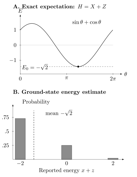
For $\lvert\psi(\theta)\rangle=R_y(\theta)\lvert0\rangle$ and $H=X+Z$, the exact energy is $E(\theta)=\sin\theta+\cos\theta\ge-\sqrt2$. At the minimizing angle, independently measuring each Pauli term once produces the lower panel’s distribution. Its mean is $-\sqrt2$, although its most likely reported value is $-2$. These are probabilities from the specified ideal experiment, not simulated training data.

The intrinsic energy variance of this exact ground state is zero, whereas the two-shot estimator has variance one in these energy units. Hamiltonian variance and the sampling variance of an estimator assembled from separate settings are different quantities.

Energy Error and State Fidelity

Assume a nondegenerate ground state and gap

$$\Delta = E_1-E_0 > 0.$$

The spectral expansion gives

$$E-E_0 \geq \Delta \left( 1-\lvert c_0\rvert^2 \right).$$

Therefore

$$\lvert \langle E_0\vert\psi\rangle \rvert^2 \geq 1- \frac{E-E_0}{\Delta}.$$

A small energy error certifies high ground-state overlap only relative to a known gap. When $\Delta$ is small, a visibly accurate energy may coexist with substantial excited-state weight. In a degenerate ground space, replace $\lvert c_0\rvert^2$ by the total weight in that space and use the gap above it.

For a mixed state, the same proof gives the ground-space probability $F_0=\operatorname{Tr}(\rho\Pi_0)$, where $\Pi_0$ projects onto the ground eigenspace. This is the squared fidelity with the ground state when it is nondegenerate.

Since $E_0$ is usually unknown, suppose we instead know a rigorous lower bound $L\le E_0$, a positive lower bound $\delta\le\Delta$ on the gap, and an upper bound $U\ge E=\operatorname{Tr}(\rho H)$ on the energy of this prepared state. Then

$$1-F_0\le\frac{E-E_0}{\Delta} \le\frac{U-L}{\delta}.$$

An upper bound on $E_0$ alone is insufficient: for $H=\operatorname{diag}(0,1)$, the interval $L=U=0$ identifies the ground energy exactly but says nothing about a preparation of the excited state. If $U$ is a statistical confidence bound, the fidelity conclusion holds with the confidence of the required joint bounds, and only after any systematic bias has been bounded.

For example, $L=-1.415$, $U=-1.390$ and $\delta=2.8$ give $F_0\ge0.99107$. The energy units must agree. The lower bound $\delta$, not an unverified estimate of the gap, is what makes the conclusion conservative.

Energy variance

The energy variance is

$$\sigma_H^2 = \langle H^2\rangle - \langle H\rangle^2.$$

It vanishes exactly when the state has support inside one eigenspace. A small variance indicates concentration near one or more nearby eigenvalues, but does not by itself identify the ground state. Measuring $H^2$ can also be expensive: the product of two Pauli sums may contain many terms even after algebraic simplification.

A Four-Part VQE Error Budget

Let $E_\Theta=\inf_{\theta\in\Theta}E(\theta)$ and let $\widehat\theta$ be the selected parameters. Denote the mean of the actual measurement procedure by $E_{\rm phys}(\widehat\theta)$ and its reported finite-data estimate by $\widehat E$. Adding and subtracting the intermediate quantities gives

$$\widehat E-E_0={}(\widehat E-E_{\rm phys}) +[E_{\rm phys}-E(\widehat\theta)] +[E(\widehat\theta)-E_\Theta] +(E_\Theta-E_0).$$

Using an infimum keeps this decomposition valid even when the family approaches its best state only in a limit.

The terms are:

1. statistical and analysis error in the reported estimator;
2. implementation error from noise, drift, readout, compilation, and observable mismatch;
3. optimization error within the chosen family;
4. representation error of the family itself.

For chemistry, a fifth layer sits outside this equation: model error between $E_0$ of the encoded Hamiltonian and the desired physical quantity. Basis truncation, active spaces, frozen cores, relativistic effects, Born–Oppenheimer separation, and geometry all contribute.

These terms need not have fixed signs. The ideal optimization and representation terms are nonnegative. Statistical fluctuations, mitigation, and model differences can be positive or negative.

From a Physical Problem to a Qubit Hamiltonian

VQE solves the operator it is given. For a molecular calculation at fixed nuclear geometry, a common second-quantized electronic Hamiltonian is

$$H_{\mathrm e} = E_{\mathrm{nn}} + \sum_{p,q} h_{pq} a_p^\dagger a_q + \frac12 \sum_{p,q,r,s} h_{pqrs} a_p^\dagger a_q^\dagger a_s a_r.$$

Here the one- and two-electron integrals depend on the orbital basis and nuclear geometry, while $E_{\mathrm{nn}}$ is the nuclear repulsion energy. Here $h_{pqrs}$ denotes the unsymmetrized two-particle matrix element $\langle p,q\lvert v\rvert r,s\rangle$ in orthonormal spin orbitals. The factor $1/2$ is consistent with that convention; antisymmetrized integrals instead use a $1/4$ coefficient with the corresponding full index sum. Many-particle Hamiltonians derives the operator, and electronic structure explains the physical approximations.

A fermion-to-qubit transformation produces

$$H_{\mathrm q} = \sum_{j=0}^{M-1} h_j P_j,$$

where each $P_j$ is an $n$-qubit Pauli word. Jordan–Wigner, parity, and Bravyi–Kitaev-type encodings differ in locality, symmetry exposure, and compilation cost. Qubit tapering can remove fixed symmetry sectors. These transformations must preserve the intended spectrum within the selected sector; a smaller qubit count is not useful if the wrong charge, spin, or parity sector is retained.

Constant shifts affect reported absolute energies even when they do not change the trial state. Fix the orbital basis, particle number, geometry and units before comparing two methods. Simulation of quantum chemistry follows the construction from molecular integrals to a qubit Hamiltonian; simulation of quantum materials treats lattice and periodic models. For spin models the Hamiltonian may already be expressed as Pauli operators.

Choosing the Trial Family

The ansatz must balance reachability, circuit cost, symmetry, and trainability. No family is uniformly best.

Reference states

For weakly correlated molecular regimes, the Hartree–Fock determinant is a common reference. It is easy to prepare in an occupation encoding and fixes particle number. Near bond dissociation, transition-metal complexes, or other strongly correlated regimes, a single determinant can have poor overlap with the target. Multireference, active-space, tensor-network, or classically preoptimized references may then be more appropriate.

A strong classical reference is not an unfair shortcut. It is part of the hybrid algorithm and must be included in the cost and comparator. If the classical procedure already returns the desired energy and observables, the incremental role of the quantum step must be stated.

Unitary coupled cluster

For occupied orbitals $i,j$ and virtual orbitals $a,b$, define

$$T = T_1+T_2+\cdots,$$

with

$$T_1 = \sum_{i,a} t_i^a a_a^\dagger a_i,$$

and

$$T_2 = \frac14 \sum_{i,j,a,b} t_{ij}^{ab} a_a^\dagger a_b^\dagger a_j a_i.$$

The unitary coupled-cluster state is

$$\lvert\psi_{\mathrm{UCC}}\rangle = e^{T-T^\dagger} \lvert\psi_{\mathrm{ref}}\rangle.$$

The normalized state gives a variational energy, unlike the usual projected energy of conventional nonunitary coupled cluster. On a gate model, the excitation generator is mapped to Pauli operators and usually decomposed or product-formula approximated. Ordering, repetitions, compilation, and parameter reoptimization define the actual circuit family. A product of unitary factors still gives a variational expectation of the same $H$, even when it approximates the intended UCC unitary poorly; the approximation changes the family, not Rayleigh–Ritz. UCC singles and doubles can be chemically structured but deep, and truncated excitation rank can fail in strongly correlated regimes.

Hardware-efficient families

Hardware-efficient VQE alternates native rotations and entangling layers. These circuits can be shallow after compilation and were important in early experiments. They need not conserve particle number or spin, and increasing generic expressibility can worsen trainability. Use explicit penalties or, preferably when practical, symmetry-preserving gates and references.

Symmetry-preserving families

If

$$[H,S_\alpha]=0,$$

the search can be restricted to a compatible common eigenspace when the selected $S_\alpha$ commute with one another as well as with $H$. This reduces irrelevant directions and enables symmetry verification. The restriction is valid only when the desired ground state lies in that sector. Along a molecular geometry scan, state crossings can change which sector or root is physically relevant.

Adaptive families

ADAPT-style VQE begins from a reference and appends operators from a pool. For an anti-Hermitian candidate $A_\mu$, the initial energy derivative is

$$\left. \frac{d}{d\theta} \langle e^{-\theta A_\mu} H e^{\theta A_\mu} \rangle \right|_{\theta=0} = \langle [H,A_\mu] \rangle.$$

The candidate with a large measured gradient is appended, all parameters are reoptimized, and growth continues until a stopping criterion fires. Adaptive construction can produce compact circuits, but screening every pool operator adds measurement and selection cost. The operator pool and uncertainty of its gradient estimates matter. Vanishing pool gradients do not certify a ground state: every exact energy eigenstate has $\langle[H,A]\rangle=0$ for every $A$, including excited eigenstates. For $H=Z$, the excited state $\lvert0\rangle$ has $E(\theta)=\cos\theta$ under a $Y$ rotation. Its gradient vanishes at zero even though any small nonzero rotation lowers its energy. Curvature, a finite trial step or a changed reference can reveal the problem.

Estimating the Energy

For

$$H = \sum_j h_jP_j,$$

linearity gives

$$E(\boldsymbol{\theta}) = \sum_j h_j \mu_j(\boldsymbol{\theta}), \qquad \mu_j = \langle P_j\rangle.$$

Each Pauli word has outcomes $\pm1$, so an independent sample mean from $N_j$ shots has

$$\operatorname{Var}(\widehat\mu_j) = \frac{1-\mu_j^2}{N_j}.$$

If every term is measured separately,

$$\operatorname{Var}(\widehat E) = \sum_j \frac{ h_j^2 \left( 1-\mu_j^2 \right) }{ N_j }.$$

For a fixed total shot count and known variances, the continuous optimum is

$$N_j \propto \lvert h_j\rvert \sqrt{1-\mu_j^2}.$$

A zero-variance term needs no further shots only if its mean is already known; zero variance inferred from a small pilot sample is not proof of determinism. The variances change with $\boldsymbol{\theta}$, so pilot measurements or adaptive allocation can outperform a fixed uniform schedule. Shot allocation must not be optimized on the final data without accounting for that adaptivity.

Grouping compatible terms

Commuting Pauli words can sometimes be measured in one basis. Qubit-wise commuting groups require only local basis changes; general commuting groups may need entangling diagonalization circuits. For group $g$, one shot produces several correlated Pauli outcomes, so

$$\operatorname{Var}(\widehat E_g) = \frac1{N_g} \sum_{j,k\in g} h_jh_k \operatorname{Cov}(P_j,P_k).$$

Minimizing the number of groups is not equivalent to minimizing energy variance or wall time. Larger groups can add basis-change depth, crosstalk, and covariance. A measurement design should optimize the implemented variance-cost tradeoff. Crawford and collaborators analyze finite-sampling measurement costs, while Huggins and collaborators develop chemistry-specific basis rotations.

For a simple covariance example, the state $(\lvert01\rangle+\lvert10\rangle)/\sqrt2$ has individually random $Z_0$ and $Z_1$ outcomes but always $Z_0+Z_1=0$. Measuring both in the same shot gives a zero-variance estimate of their sum. Measuring them on independent preparations loses that anticorrelation and gives variance $2/N$ when each term receives $N$ shots. The grouping advantage here follows from the covariance, not just the reduced number of settings.

Fermionic and low-rank measurement structure

Molecular two-electron tensors have algebraic structure that can be factorized. Basis-rotation and low-rank schemes measure families of number operators after orbital rotations, potentially reducing the number of settings and mitigating long parity strings. They exchange measurement count for additional coherent depth and model-specific preprocessing. Compare total state preparations, compiled gates, variance, and bias rather than settings alone.

Optimizing the Energy

VQE optimization is unusually coupled to measurement design. The objective is not merely noisy: its variance depends on the state, shot allocation, measurement grouping, compilation, and hardware drift. Two evaluations at different parameters therefore need not have equal precision. An optimizer that interprets every fluctuation as objective structure can spend most of its budget chasing shot noise.

Variational quantum algorithms explains optimizers and gradient estimators. For energy minimization, compare proposed changes with their uncertainty and distinguish the best value found during search from a fresh estimate at the selected parameters. Symmetries and energy variance provide additional information, but neither replaces an energy comparison with a trustworthy bound or tractable exact solution.

Initialization and continuation

Starting near a suitable physical reference can reduce the search effort. A good initial state still needs enough flexibility to describe changes such as bond breaking.

For a sequence of nearby Hamiltonians $H(R)$, such as points along a molecular geometry coordinate $R$, parameters from one point can initialize the next. This continuation strategy often lowers search cost, but it can also remain on a metastable branch through an avoided crossing or symmetry change. Geometry order, forward and reverse sweeps, discontinuities, and fallback initializations should therefore be reported.

Gradients and stopping

If the ansatz gate generators admit a parameter-shift rule, derivatives of the VQE energy can be estimated from shifted energy evaluations. The same Hamiltonian measurement problem is then repeated for every shifted circuit. Analytic gradients remove finite-difference truncation error, but not sampling noise, hardware bias, or the multiplicative cost in parameter count.

A small measured gradient is not by itself evidence of convergence. It may indicate an optimum, a barren plateau, excessive shot noise, or a parameter redundancy. A defensible stopping rule combines several signals, for example:

$$\begin{aligned} \lvert \widehat E_{t} - \widehat E_{t-1} \rvert &\lesssim \tau_E, \\ \lVert \widehat{\boldsymbol{\nabla}}E_t \rVert &\lesssim \tau_g, \\ \widehat{\operatorname{SE}} \left( \widehat E_t \right) &\lesssim \tau_{\mathrm{stat}}, \end{aligned}$$

for several iterations, followed by a fresh validation run. These are stopping diagnostics rather than a proof of global optimality. Correlated estimates and repeated testing require uncertainty rules appropriate to the sampling procedure.

Worked Two-Qubit Reduction

Consider the real, number-conserving Hamiltonian

$$H ={} \alpha I + \beta Z_0 + \gamma Z_1 + \delta Z_0Z_1 + \frac{\kappa}{2} \left( X_0X_1 + Y_0Y_1 \right).$$

Use the tensor order $\lvert q_0q_1\rangle$, so $Z_0=Z\otimes I$ and $Z_1=I\otimes Z$. Restrict attention to the one-excitation sector and prepare

$$\lvert\psi(\theta)\rangle = \cos\frac{\theta}{2} \lvert01\rangle + \sin\frac{\theta}{2} \lvert10\rangle.$$

The required expectation values are

$$\begin{aligned} \langle Z_0\rangle &= \cos\theta, & \langle Z_1\rangle &= -\cos\theta, \\ \langle Z_0Z_1\rangle &= -1, & \langle X_0X_1\rangle &= \sin\theta, \\ \langle Y_0Y_1\rangle &= \sin\theta. \end{aligned}$$

Thus the entire VQE objective is the sinusoid

$$E(\theta) = \alpha-\delta + \left( \beta-\gamma \right) \cos\theta + \kappa\sin\theta.$$

Its exact minimum within this sector is

$$E_{\mathrm{sector}} = \alpha-\delta - \sqrt{ \left( \beta-\gamma \right)^2 + \kappa^2 }.$$

For $(\alpha,\beta,\gamma,\delta,\kappa)=(0,0.4,-0.1,0.2,0.3)$, the sector minimum is $-0.2-\sqrt{0.34}\approx-0.783095$. The other two sectors contain $\lvert00\rangle$ and $\lvert11\rangle$ with energies $\alpha+\beta+\gamma+\delta=0.5$ and $\alpha-\beta-\gamma+\delta=-0.1$, so this sector does contain the global ground state. Changing only $\delta$ to $-1$ puts the global minimum at $\lvert11\rangle$ with energy $-1.3$, below the one-excitation minimum $1-\sqrt{0.34}\approx0.416905$.

This example separates a correct optimization within a sector from selecting the correct sector. The $Z$-type terms share one local measurement basis. The two exchange terms commute, although measuring them together may require an entangling diagonalization; separate $X$ and $Y$ bases are simpler. The ansatz explores the real one-excitation subspace, the symmetry sector is exact, and the analytic sector minimum gives an independent benchmark for the optimizer and estimator. If the global ground state lies in a different excitation sector, however, the sector minimum remains an upper bound rather than the global answer.

Noise, Mitigation, and the Variational Bound

The mixed-state proof above assumes exact measurements of $H$ on a common physical state. Preparation errors satisfy that premise if they produce one normalized density operator. Readout bias, basis-dependent control errors and drift can instead change the measured operator or make different settings sample different states. More shots then resolve the wrong mean more precisely.

An estimate below a trustworthy $E_0$ therefore calls for a check of its statistical uncertainty and measurement assumptions. It is not a state with energy below the ground state.

Mitigation inside an adaptive loop

Symmetry verification can physically condition on an accepted sector, in which case the normalized conditional state remains variational. A ratio assembled from estimated expectation values need not obey the bound on every realization. Zero-noise extrapolation and probabilistic error cancellation can use signed combinations of data that do not themselves represent a physical density operator. Their bias and uncertainty must be assessed separately.

Applying mitigation at every optimizer step can be prohibitively expensive. Applying it only to the final point can instead select parameters using a different objective from the one ultimately reported. A useful compromise is to use a stable low-cost protocol during search, validate several candidates with a higher-fidelity protocol, and use independent data for the final selected candidate. Noise in quantum information explains the channel and measurement models.

Selection bias

Suppose $M$ candidate parameters have the same true energy and independent zero-mean estimator noise. Selecting the smallest observed value makes the selected estimate downward biased even though every individual estimator is unbiased. The effect grows with $M$ and with estimator variance. Consequently, the minimum value seen during optimization is not a valid final estimate. Reprepare the selected state and collect independent validation data.

Chemical Accuracy and Model Accuracy

In quantum chemistry, chemical accuracy conventionally means roughly $1\,\mathrm{kcal\,mol^{-1}}$:

$$1\,\mathrm{kcal\,mol^{-1}} \approx 1.5936\times10^{-3}\,E_{\mathrm h} \approx 0.04336\,\mathrm{eV}.$$

This threshold is a historical heuristic, not a universal criterion for chemical usefulness. Reaction energies, barrier heights, spin gaps, spectroscopic splittings, and response properties can require different accuracy. Moreover, reaching this tolerance relative to the exact ground energy of a small active-space Hamiltonian does not imply the same accuracy relative to experiment.

It is clearer to distinguish:

• algorithmic accuracy relative to the exact eigenvalue of the encoded finite Hamiltonian;
• electronic-structure model error from basis truncation, frozen orbitals, active-space choice, and correlation approximations;
• physical-model error from geometry, relativity, nonadiabatic effects, environment, and omitted interactions;
• experimental uncertainty in the quantity used for comparison.

Energy differences also require consistent models. Two absolute energies can share large correlated errors that cancel, while separately chosen active spaces can create an artificial difference. The Electronic Structure Overview explains these modeling approximations.

Excited States and Subspace Methods

The basic variational principle targets the lowest state available in the chosen symmetry sector. Excited-state algorithms modify the objective or solve a projected eigenproblem, and therefore have different guarantees.

Variational deflation

After approximating lower states $\lvert\widetilde\psi_j\rangle$, one can minimize

$$C_k(\boldsymbol{\theta}) = \langle H\rangle_{\boldsymbol{\theta}} + \sum_{j<k} \lambda_j \left| \langle \widetilde\psi_j \vert \psi(\boldsymbol{\theta}) \rangle \right|^2.$$

For exact orthonormal lower eigenstates, each penalty shifts only its own level: $E_j\mapsto E_j+\lambda_j$. Taking $\lambda_j>E_k-E_j$ for every $j<k$ makes the $k$th level a ground level of the penalized operator; target degeneracies can remain. Higgott, Wang and Brierley develop this deflation method. In practice, imperfect lower states, uncertain overlaps, and poorly chosen penalties can distort the spectrum. A large penalty cannot repair an incorrect lower-state projector. For $H=\operatorname{diag}(0,\Delta)$ and an approximate lower state $\cos\eta\lvert0\rangle+\sin\eta\lvert1\rangle$, the lowest penalized state approaches its orthogonal vector as $\lambda\to\infty$. Its expectation of the original $H$ approaches $\Delta\cos^2\eta$, not $\Delta$. The finite error is due to the incorrect orthogonality constraint.

Quantum subspace expansion

Choose states

$$\lvert\phi_a\rangle = O_a \lvert\psi\rangle$$

generated from a prepared reference by excitation or response operators. Measure

$$H_{ab} = \langle\phi_a\rvert H\lvert\phi_b\rangle, \qquad S_{ab} = \langle\phi_a\vert\phi_b\rangle,$$

and solve the generalized eigenproblem

$$H\boldsymbol{c} = E S\boldsymbol{c}.$$

With exact matrices, discard null directions of $S$ and transform to an orthonormal basis of the span. The resulting Hermitian projected Hamiltonian obeys the Rayleigh–Ritz min–max principle: its ordered Ritz values $\varepsilon_j$ satisfy $\varepsilon_j\ge E_j$ of the full Hamiltonian, for as many directions as the subspace contains. This is a genuine variational property of the exact projected problem, not only a ground-state statement. McClean and collaborators develop quantum subspace expansion.

Shot noise can make the estimated $S$ indefinite or nearly singular. Even enforcing a positive estimated $S$ does not restore variationality unless the estimated matrices consistently describe a true subspace of the same $H$. Small overlap eigenvalues amplify measurement errors; truncating those directions changes the retained subspace and can improve stability at the cost of flexibility.

State-averaged, contracted, and equation-of-motion variants make different tradeoffs among orthogonality, measurement cost, and accessible excitations. None should be described as inheriting the ground-state VQE upper bound without a separate proof.

VQE and Phase Estimation

VQE and Quantum Phase Estimation solve related spectral problems with different resource assumptions.

VQE estimates many expectation values by repeated state preparation. Plain sampling to additive standard error $\epsilon$ typically has $O(\epsilon^{-2})$ shot scaling, before accounting for Hamiltonian size, optimization, or mitigation. It tolerates short circuits but can demand many adaptive repetitions.

Phase estimation instead uses coherent controlled evolution and can achieve $O(\epsilon^{-1})$ scaling in ideal evolution-query complexity. It requires substantial coherent depth, a state with target-eigenstate overlap, and a costly implementation of controlled dynamics. Comparing only $\epsilon^{-2}$ with $\epsilon^{-1}$ is therefore incomplete. A fair comparison compiles both methods for the same Hamiltonian, error target, success probability, hardware model, and state-preparation assumptions.

Measurement cost and useful accuracy

If $N_{t,g}$ preparations are used for measurement group $g$ at parameter evaluation $t$, objective evaluations consume $\sum_{t,g}N_{t,g}$ preparations. Add gradient, overlap, calibration and mitigation circuits, unsuccessful restarts and final measurements exactly once. For example, 200 evaluations of 20 groups with 1,000 shots per group use four million preparations before these additions. At a hypothetical one millisecond per preparation, that alone is about 67 minutes, even if each coherent circuit is short. Parallel operation and hardware latency change the elapsed time.

Compare methods for the same Hamiltonian, sector, accuracy and output. A ground-energy estimate, a prepared ground state and a chemical energy difference have different requirements. Exact diagonalization on small models checks the encoding and optimization, while stronger classical methods on larger models test whether a quantum step improves the achieved accuracy or cost. Algorithmic benchmarking and resource estimation develop these comparisons.

Common pitfalls

A small statistical error is not a small total error. More shots reduce uncertainty around the implemented mean. They do not enlarge the ansatz, correct the molecular model or remove an unbounded calibration bias.

Zero energy variance does not identify the ground state. Every excited eigenstate also has zero variance. Ground-state overlap requires additional spectral or state information.

The lowest observed sample is selected data. Comparing many noisy estimates tends to favor an unusually low fluctuation. Reprepare the selected state and estimate its energy independently; retain uncertainty in that final answer.

Further directions

VQE combines an exact variational statement with approximation, optimization and measurement tasks whose difficulty depends on the model and implementation. An expressive state family need not be easy to optimize, and a precise estimate need not be physically accurate. These distinctions remain useful as devices and methods change. Quantum chemistry at scale discusses dated research questions and feasibility assessments.

For physical applications, quantum chemistry case studies and simulation of quantum materials explain how an energy calculation supports a scientific question. Hybrid quantum simulation treats time evolution and embedding methods that can use a VQE state as an ingredient.

Exercises

1. Mixed-state variational bound

Let $\rho$ be any density operator and let $E_0$ be the lowest eigenvalue of $H$. Prove that $\operatorname{Tr}(\rho H)\geq E_0$. Explain why a finite-shot energy estimate can nevertheless lie below $E_0$.

Solution

In the energy eigenbasis, define

$$p_k = \langle E_k\rvert\rho\lvert E_k\rangle.$$

Positivity and unit trace give $p_k\geq0$ and $\sum_kp_k=1$. Therefore

$$\operatorname{Tr}(\rho H) = \sum_kp_kE_k \geq E_0\sum_kp_k = E_0.$$

A finite-shot estimator is a random variable centered on the expectation only under an unbiased protocol. Even then, individual realizations can fall on either side of the mean. Readout bias, mitigation, and selection of the smallest observed value can produce additional downward displacement.

2. Energy error and overlap

Assume a nondegenerate ground state and a gap $\Delta=E_1-E_0>0$. Show that a normalized state with energy $E_\psi$ satisfies

$$1- \left| \langle E_0\vert\psi\rangle \right|^2 \leq \frac{E_\psi-E_0}{\Delta}.$$

Why can a small energy error be a weak fidelity certificate?

Solution

Writing $\lvert\psi\rangle=\sum_kc_k\lvert E_k\rangle$ gives

$$\begin{aligned} E_\psi-E_0 &= \sum_{k>0} \lvert c_k\rvert^2 \left( E_k-E_0 \right) \\ &\geq \Delta \sum_{k>0} \lvert c_k\rvert^2. \end{aligned}$$

The sum is $1-\lvert\langle E_0\vert\psi\rangle\rvert^2$, which proves the result. When $\Delta$ is small, dividing by the gap gives a loose bound: appreciable excited-state weight can cost little energy.

3. Optimal independent shot allocation

For independent Pauli estimates with variances $v_j/N_j$, minimize

$$\sum_j \frac{h_j^2v_j}{N_j}$$

subject to $\sum_jN_j=N$. Treat $N_j$ as continuous.

Solution

Introduce a multiplier $\lambda$:

$$\mathcal L = \sum_j \frac{h_j^2v_j}{N_j} + \lambda \left( \sum_jN_j-N \right).$$

Stationarity gives

$$N_j = \frac{ \lvert h_j\rvert \sqrt{v_j} }{ \sqrt{\lambda} }.$$

After normalization,

$$N_j = N \frac{ \lvert h_j\rvert\sqrt{v_j} }{ \sum_k \lvert h_k\rvert\sqrt{v_k} }.$$

Integer rounding, pilot-shot floors, grouping covariance, and changing variances make the implemented allocation an adaptive approximation to this ideal result.

4. Solve the two-qubit model

Derive the objective for the two-qubit state in the worked example and find an angle attaining the sector minimum.

Solution

The expectation values listed above give

$$E(\theta) = C + A\cos\theta + \kappa\sin\theta,$$

where $C=\alpha-\delta$ and $A=\beta-\gamma$. Write

$$A\cos\theta + \kappa\sin\theta = R\cos(\theta-\phi),$$

with

$$R = \sqrt{A^2+\kappa^2}, \qquad \phi = \operatorname{atan2}(\kappa,A).$$

Any $\theta_\star=\phi+\pi$ modulo $2\pi$ attains $E_{\mathrm{sector}}=C-R$.

5. Selection bias

Two candidate parameter settings have the same true energy $E$. Their search estimates are $\widehat E_i=E+\varepsilon_i$, where the $\varepsilon_i$ are independent zero-mean Gaussian variables with standard deviation $\sigma$. Is $\min(\widehat E_1,\widehat E_2)$ unbiased? Give a qualitative remedy.

Solution

It is downward biased. Using

$$\min(x,y) = \frac{x+y-\lvert x-y\rvert}{2}$$

gives

$$\mathbb E \left[ \min(\widehat E_1,\widehat E_2) \right] = E - \frac12 \mathbb E \left[ \lvert\varepsilon_1-\varepsilon_2\rvert \right] < E.$$

For Gaussian noise the bias equals $-\sigma/\sqrt{\pi}$. Select candidates using the search data, then estimate the chosen candidate’s energy with fresh, independent validation shots. The validation uncertainty remains, but the reported mean no longer reuses the selection fluctuation.

6. Variational deflation penalty

Suppose the exact ground state is known and define

$$H' = H + \lambda \lvert E_0\rangle\langle E_0\rvert.$$

What condition on $\lambda$ makes $\lvert E_1\rangle$ a ground state of $H'$?

Solution

The eigenvalues of $H'$ are $E_0+\lambda$ for the original ground state and $E_k$ for every $k>0$. Therefore $\lvert E_1\rangle$ is a ground state when

$$E_1 \leq E_0+\lambda,$$

or $\lambda\geq E_1-E_0$. A strict inequality removes degeneracy with the penalized ground state. Approximate lower states introduce off-diagonal distortions, so this ideal threshold does not by itself guarantee success in an experiment.

7. Model error versus algorithmic error

A VQE estimate is within $0.5\,\mathrm{kcal\,mol^{-1}}$ of exact diagonalization for its active-space Hamiltonian, while the active-space exact energy differs from a converged classical calculation by $8\,\mathrm{kcal\,mol^{-1}}$. Which accuracy claim is justified?

Solution

The stated comparison demonstrates sub-chemical algorithmic error for the encoded active-space Hamiltonian. It does not demonstrate chemical accuracy relative to the converged electronic-structure model or experiment. The dominant error is model-space error. If the $0.5$ tolerance is an absolute bound, the triangle inequality places the discrepancy from the converged calculation between $7.5$ and $8.5\,\mathrm{kcal\,mol^{-1}}$. This does not yet quantify the discrepancy from experiment.

8. Test an energy-based fidelity statement

For $H=\operatorname{diag}(0,1)$, someone knows the exact ground energy and sets $L=U=0$. They infer unit ground-state fidelity from $1-F_0\le(U-L)/\Delta$. What assumption is missing? Give a correct statement with statistical energy information.

Solution

The prepared state could be $\lvert1\rangle$, with energy one and ground-state fidelity zero. Knowing $E_0$ does not bound that state’s energy from above. The missing condition is $U\ge\operatorname{Tr}(\rho H)$, not merely $U\ge E_0$.

If independent measurements give an upper confidence bound $U=0.03$ on the prepared state’s true energy with coverage at least $0.95$, and systematic bias has been bounded, then $L=0$ and $\Delta=1$ give $F_0\ge0.97$ with at least that coverage. The conclusion concerns the particular state sampled by those measurements, assuming a stable preparation. For a degenerate ground level it instead bounds total probability in the ground eigenspace.

References

• O. Crawford et al., “Efficient quantum measurement of Pauli operators in the presence of finite sampling error,” Quantum 5, 385 (2021), doi:10.22331/q-2021-01-20-385.
• B. T. Gard et al., “Efficient symmetry-preserving state preparation circuits for the variational quantum eigensolver algorithm,” npj Quantum Information 6, 10 (2020), doi:10.1038/s41534-019-0240-1.
• H. R. Grimsley et al., “An adaptive variational algorithm for exact molecular simulations on a quantum computer,” Nature Communications 10, 3007 (2019), doi:10.1038/s41467-019-10988-2.
• O. Higgott, D. Wang, and S. Brierley, “Variational quantum computation of excited states,” Quantum 3, 156 (2019), doi:10.22331/q-2019-07-01-156.
• W. J. Huggins et al., “Efficient and noise resilient measurements for quantum chemistry on near-term quantum computers,” npj Quantum Information 7, 23 (2021), doi:10.1038/s41534-020-00341-7.
• A. Kandala et al., “Hardware-efficient variational quantum eigensolver for small molecules and quantum magnets,” Nature 549, 242–246 (2017), doi:10.1038/nature23879.
• S. McArdle et al., “Quantum computational chemistry,” Reviews of Modern Physics 92, 015003 (2020), doi:10.1103/RevModPhys.92.015003.
• J. R. McClean et al., “Hybrid quantum-classical hierarchy for mitigation of decoherence and determination of excited states,” Physical Review A 95, 042308 (2017), doi:10.1103/PhysRevA.95.042308.
• J. R. McClean et al., “The theory of variational hybrid quantum-classical algorithms,” New Journal of Physics 18, 023023 (2016), doi:10.1088/1367-2630/18/2/023023.
• A. Peruzzo et al., “A variational eigenvalue solver on a photonic quantum processor,” Nature Communications 5, 4213 (2014), doi:10.1038/ncomms5213.
• J. Romero et al., “Strategies for quantum computing molecular energies using the unitary coupled cluster ansatz,” Quantum Science and Technology 4, 014008 (2018), doi:10.1088/2058-9565/aad3e4.
• R. Sagastizabal et al., “Experimental error mitigation via symmetry verification in a variational quantum eigensolver,” Physical Review A 100, 010302(R) (2019), doi:10.1103/PhysRevA.100.010302.
• H. L. Tang et al., “qubit-ADAPT-VQE: an adaptive algorithm for constructing hardware-efficient ansätze on a quantum processor,” PRX Quantum 2, 020310 (2021), doi:10.1103/PRXQuantum.2.020310.
• K. Temme, S. Bravyi, and J. M. Gambetta, “Error mitigation for short-depth quantum circuits,” Physical Review Letters 119, 180509 (2017), doi:10.1103/PhysRevLett.119.180509.
• J. Tilly et al., “The variational quantum eigensolver: a review of methods and best practices,” Physics Reports 986, 1–128 (2022), doi:10.1016/j.physrep.2022.08.003.
• V. Verteletskyi, T.-C. Yen, and A. F. Izmaylov, “Measurement optimization in the variational quantum eigensolver using a minimum clique cover,” Journal of Chemical Physics 152, 124114 (2020), doi:10.1063/1.5141458.