Resource Estimation Tools

A quantum resource estimator translates an application into requirements such as logical gates, peak qubits, error-correction cycles, and runtime under a chosen machine model. The answer depends on the input problem, required accuracy, circuit construction, and hardware assumptions. An exact gate count can feed an uncertain physical estimate.

This page explains how to use and compare these tools, with a worked example showing why factory count, code distance, and runtime must be evaluated together. Resource estimation develops the underlying fault-tolerant cost model; here the emphasis is on turning a program and its assumptions into a calculation that can be checked and varied.

Helpful background. The quantum software stack connects programs to hardware. Circuit intermediate representations explains gates, qubit lifetimes, and classical branches. The surface code introduces code distance and repeated syndrome measurements.

Logical programs and resource counts

Start by fixing the task: which instance is solved, what output is needed, and what accuracy and success probability are required? A phase-estimation subroutine alone does not include state preparation, imperfect initial overlap, retries, or classical processing. These can dominate the application.

Different stages of an estimate answer different questions.

Stage	Typical answer	Additional assumptions
Algorithm scaling	Queries as size grows	Input access and precision
Logical program	Gates, depth, peak live qubits	Decomposition and gate basis
Fault-tolerant model	Distances, factories, cycles	Code, decoder, logical operations
Physical schedule	Qubits and elapsed time	Layout, delivery, control latency

These stages are not unit conversions. An oracle must become a reversible circuit; a rotation must become an allowed gate sequence; a logical operation must become a protected protocol. Beverland and colleagues describe a layered estimation framework that makes these choices explicit.

Count the leaves of a call graph

Suppose subroutine $b$ is called $m_b$ times and costs $c_{b,g}$ primitive gates of type $g$. For a chosen non-overlapping set of subroutine calls,

$$N_g=\sum_b m_b c_{b,g}.$$

When expanding a hierarchical call graph, count the selected leaves once. Adding a subroutine’s already-expanded total to all of its children’s totals counts the same operations twice. Distinguish a cost supplied by an analytic formula from one obtained by decomposing a concrete circuit. Both can be useful, but their agreement on small instances is a valuable check.

Harrigan and colleagues develop this approach in Qualtran. Its call-graph documentation explains explicit cost annotations, fallback to decompositions, and comparison of the two. A stored cost is not itself a functional test of the circuit.

Counts, depth, and live qubits

Gate count measures total work. Dependency depth measures sequential layers. Neither alone determines runtime when gates compete for routing space, measurements, or resource states. Likewise, the peak logical workspace is

$$Q_{\mathrm{log,peak}} =\max_t[Q_{\mathrm{data}}(t)+Q_{\mathrm{work}}(t)].$$

Sequential subroutines can reuse clean ancillas. An ancilla that remains entangled with live data cannot simply be relabeled as a fresh $\lvert0\rangle$; uncomputation or reset may cost gates and time. On branching programs, average width is a workload statistic, not enough capacity to execute every branch. For example, equiprobable branches needing 10 or 100 live qubits have average width 55, but a machine that must support both needs at least 100.

State the gate basis and approximation precision beside the count. An arbitrary rotation and a synthesized Clifford+$T$ sequence are different units. Gate decomposition explains this conversion, including when phases become relevant to controlled operations.

Accuracy, failure, and repeated attempts

For unitary gates whose operator-norm errors are bounded by $\epsilon_r$, a telescoping product gives the sufficient synthesis condition

$$\sum_r\epsilon_r\leq\epsilon_{\mathrm{syn}}.$$

This assumes the norms compare the actual operations used, with consistent phase conventions. An energy bias, average gate infidelity, and probability of a logical fault cannot simply be added to this norm budget.

For failure events, the union bound is

$$P(\text{at least one failure})\leq\sum_j P(E_j).$$

It does not require independence, but each event probability must be a valid bound in the modeled operating context. Substituting a phenomenological fit produces a model estimate, not a rigorous device guarantee. Exceeding a conservative upper bound’s allocated budget means that this calculation no longer certifies the target; it does not prove that the true failure rate is too high.

Ross and Selinger analyze Clifford+$T$ rotation synthesis. In a smooth toy cost model $a_r\log_2(1/\epsilon_r)$, equal error allocation is optimal when all coefficients $a_r$ are equal. With unequal coefficients and the simple sum constraint above, the unconstrained optimum assigns $\epsilon_r\propto a_r$. Physical synthesis has discrete lengths and other constraints, so the final circuit still needs to be evaluated.

Successful runs must be recognizable to stop retrying

For independent attempts with $0<p_s<1$, the probability of at least one success in $R$ attempts is $1-(1-p_s)^R$. Thus

$$R_\delta=\left\lceil \frac{\log\delta}{\log(1-p_s)}\right\rceil$$

is sufficient to obtain at least one success with probability $1-\delta$. Stopping at the first success requires a trustworthy herald or verification procedure. If correctness is unobserved, this formula alone does not identify which returned answer is correct. Correlated failures across retries also invalidate the independent-attempt formula.

For identifiable success, the expected number of attempts is $1/p_s$. If a successful attempt costs $c_s$ and a failed one costs $c_f$, the expected cost until success is

$$\mathbb E[C]=c_s+\frac{1-p_s}{p_s}c_f.$$

Early rejection can therefore matter greatly. Sampling an expectation or probability is a different task: its total cost includes the number of shots required by the chosen confidence interval, not just a success retry count.

Code distance and factory supply

A code model may assign a logical failure probability per specified protected location, often using a below-threshold fit of the form

$$p_{\mathrm L}(d)\simeq A \left(\frac{p}{p_{\mathrm{th}}}\right)^{(d+1)/2}.$$

The syndrome circuit, decoder, noise assumptions, and meaning of a location determine the fit. Fowler and colleagues discuss surface-code scaling; Litinski develops lattice-surgery space–time constructions. Their results must be applied with the corresponding operation and geometry assumptions. A typical selection criterion is $N_{\mathrm{loc}}p_{\mathrm L}(d)\leq\epsilon_{\mathrm L}$, but the location count may increase with distance-dependent runtime. Recompute the schedule when changing distance.

A physical-qubit total must include the quantum data, workspace, routing, factories, buffers, and spares that the model uses. Classical controller memory, bandwidth, and power are separate quantities; they cannot be added to a qubit count. Likewise, compute elapsed time from a schedule’s critical path. Adding feedforward latency to a runtime that already includes its stalls would count the same delay twice.

Average throughput does not resolve bursts

If each factory delivers $m_F$ usable resource states every $\tau_F$, meeting total demand $M$ in time $T$ without initial stock requires at least

$$F\geq\left\lceil\frac{M\tau_F}{m_F T}\right\rceil$$

in an ideal deterministic mean-rate model. Real acceptance failures, startup, delivery, and storage can require more. Specify whether $m_F/\tau_F$ describes attempted or accepted output; an expected rate does not guarantee a deadline. Magic-state distillation develops these resource-state requirements.

An explicit buffer rule avoids hiding stockouts. Suppose supply arrives before consumption at each tick, excess supply is discarded, and $B_k$ is the inventory before arrival. Then

$$I_k=\min(B_{\max},B_k+s_k).$$

Demand $c_k$ can proceed only if $I_k\geq c_k$, after which $B_{k+1}=I_k-c_k$. Otherwise the schedule must wait or change. Applying the capacity limit only after consumption can incorrectly use states that were already discarded. A different within-tick delivery convention is possible, but it must be stated and implemented consistently.

Worked example: recompute the whole configuration

Consider a teaching model with 120 live logical data/work qubits, $C_{\min}=8\times10^7$ dependency ticks, and demand $M=2.4\times10^8$ resource states. For supported odd distance $d$, assume

$$\begin{aligned} \tau_{\mathrm L}(d)&=(d/25)\,\mu\mathrm s,\\ n_{\mathrm L}(d)&=2d^2,\\ q_F(d)&=8d^2,\\ \tau_F(d)&=10\tau_{\mathrm L}(d). \end{aligned}$$

A factory emits one usable state per $\tau_F$. Treat

$$p_{\mathrm L}(d)=2\times10^{-13}\,10^{(25-d)/2}$$

as a per-logical-qubit-tick bound inside this illustrative model, with allocation $\epsilon_{\mathrm L}=0.003$ for protected data and work. This is not a fit to a named device. Factory-output faults and other system failures are outside this allocation.

First use a mean-rate approximation with perfect overlap of supply and computation and no startup, burst, routing, or buffer delay. Its tick count is

$$C(F)=\max\left(C_{\min},\frac{10M}{F}\right).$$

For each factory count $F$, choose the smallest supported odd $d$ satisfying $120C(F)p_{\mathrm L}(d)\leq0.003$. Then calculate

$$T=C(F)\tau_{\mathrm L}(d),$$ $$Q_{\mathrm{subtotal}}=(240+8F)d^2.$$

This qubit subtotal includes only data/work patches and factories. An actual schedule can take longer than the mean-rate time, in which case its distance and failure calculation must be repeated.

Factories	Selected distance	Qubit subtotal	Mean-rate time
10	27	233,280	259.2 s
19	27	285,768	136.4 s
20	25	250,000	120 s
30	25	300,000	80 s

At 30 factories and $d=25$, the data/work failure bound is $0.00192$. Reducing to ten factories at the same distance would give $0.00576$, so that choice fails the model’s selection rule. At $d=27$ the bound becomes $0.000576$, and the revised subtotal is 233,280 qubits. The saving relative to 30 factories is 66,720 qubits, rather than the 100,000 obtained by deleting twenty factories while incorrectly keeping everything else fixed.

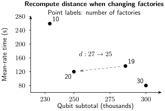
Each point recomputes distance using the same model and failure allocation. The label is the factory count. Going from 19 to 20 factories permits $d=27\to25$, reducing both modeled time and qubit subtotal. These are illustrative configurations, not hardware predictions or a complete search.

The 19-factory point is dominated by the 20-factory point: both quantities are worse. Among these four choices, 10, 20, and 30 factories are non-dominated. A Pareto frontier is always relative to the configurations searched, the objectives, and the assumptions; a heuristic search need not find the global frontier.

Choosing an estimator

The following official documentation was checked on 2026-10-15. These tools answer different parts of the calculation.

Tool	Useful question	What to inspect
Qualtran	Which subroutines and gates dominate?	Call-graph leaves and cost formulas
PennyLane estimator	What logical resources follow from this decomposition?	Gate set, precision, ancilla assumptions
Microsoft resource estimator	Which modeled physical configurations meet the budget?	QEC, factories, hardware, timing

Qualtran represents algorithms hierarchically and can connect logical counts to physical cost models. Its decomposition and count checks help locate the first disagreement between two implementations. PennyLane’s qp.estimator is specifically for logical resource estimation; its resource operators are not automatically executable compiled circuits. For a concrete compiled program, inspect the framework’s separate resource-tracking capability.

The Microsoft Quantum resource estimator combines application, architecture, error-correction/factory, and error-budget models and returns qubit–runtime tradeoffs among explored choices. Its defaults are scenarios, not measured properties of an unspecified device. An interchange format or shared gate name alone does not make two tools use the same decomposition, ancilla rules, or physical cost model.

Start with a small instance that can be hand-counted or simulated. Compare the program’s behavior and promised clean ancillas; then compare leaf counts, peak liveness, and synthesis precision. Only after those agree should you compare distances, factories, schedules, and physical totals. A tool that uses more $T$ gates and fewer ancillas may implement a legitimate space–time tradeoff rather than contain a counting error.

Vary assumptions and preserve the calculation

Separate measured parameters from fitted scaling laws, simplifying assumptions, and projected hardware targets. Explore their effect on the whole estimate. Changing a physical error rate can cross an integer distance boundary, so a small local derivative may miss the consequential change. Correlations and fit validity matter as much as a quoted error bar. Scenario labels such as optimistic and conservative are not probabilities without a justified model.

If qubit allocation changes with time, distinguish installed capacity from occupied space–time volume:

$$V=\int_0^T Q_{\mathrm{occupied}}(t)\,dt \leq Q_{\mathrm{peak}}T.$$

Releasing logical workspace may allow reuse; it does not remove fabricated qubits from the machine. State whether a qubit-hour figure counts occupied resources or reserved machine capacity.

Save the actual program or symbolic model, input parameters with units, decomposition choices, package versions, intermediate counts, and raw results alongside the plotting calculation. That is enough structure to rerun the estimate and change one assumption without reconstructing it from a headline. Keep the previous result when updating the model so the source of a changed prediction remains understandable. None of these conditional calculations, by themselves, predicts when a machine will be built.

Exercises

1. Count a hierarchical program once

A program calls $A$ three times and $B$ twice. Each $A$ calls $B$ twice and uses five additional $T$ gates; each $B$ uses seven $T$ gates. Find the total.

Solution

Each $A$ costs $2(7)+5=19$ $T$ gates, so the total is $3(19)+2(7)=71$. Equivalently, there are eight leaf calls to $B$ and fifteen additional $T$ gates: $8(7)+15=71$. Adding the expanded $A$ costs and their six internal $B$ calls again would double-count those gates.

2. Peak versus cumulative ancillas

Two sequential subroutines share $40$ data qubits. The first needs $20$ ancillas and the second needs $70$, with all ancillas released cleanly between them. What are the cumulative ancillary allocations and the minimum peak live qubits implied by this information?

Solution

The source may allocate $20+70=90$ ancillary qubits cumulatively, but the ancilla sets can reuse physical storage. The minimum peak is

$$Q_{\mathrm{peak}} = 40+\max(20,70) = 110.$$

This assumes no overlap, no routing ancillas, and immediate reuse after a verified clean release.

3. Allocate synthesis error

A simple norm budget assigns $\epsilon_{\mathrm{syn}}=10^{-3}$ across $N_R=1000$ rotations equally. What local tolerance results? In a toy cost model of $3\log_2(1/\epsilon_r)$ $T$ gates per rotation, estimate the total $T$ count.

Solution

Equal allocation gives

$$\epsilon_r = \frac{10^{-3}}{1000} = 10^{-6}.$$

Since $\log_2(10^6)\simeq19.93$, the toy model gives approximately

$$N_T \simeq 1000(3)(19.93) \simeq 5.98\times10^4.$$

Rounding a synthesis length to an allowed integer sequence would give about $60{,}000$ $T$ gates. The coefficient is part of the toy model, not a universal synthesis law.

4. Select a code distance

Assume the illustrative fit

$$p_{\mathrm L}(d) = 0.1 \left(0.1\right)^{(d+1)/2}.$$

For $N_{\mathrm{loc}}=10^9$ protected locations and logical-failure budget $10^{-3}$, find the smallest odd distance satisfying the union-bound rule.

Solution

The per-location target is

$$p_{\mathrm L} \leq \frac{10^{-3}}{10^9} = 10^{-12}.$$

The model is

$$p_{\mathrm L}(d) = 10^{-(d+3)/2}.$$

Thus $(d+3)/2\geq12$, or $d\geq21$. The smallest allowed odd distance is $d=21$. This answer is conditional on the stated fit and location definition.

5. Count average-rate factories

An application consumes $M=6.0\times10^7$ resource states in $T_{\mathrm{alg}}=30\,\mathrm{s}$. Each factory emits one state every $15\,\mu\mathrm{s}$. What average-rate lower bound follows for the number of factories?

Solution

The bound is

$$\begin{aligned} F_{\min} &= \left\lceil \frac{ (6.0\times10^7)(15\times10^{-6}\,\mathrm{s}) }{ 30\,\mathrm{s} } \right\rceil \\ &= \lceil30\rceil =30. \end{aligned}$$

This does not prove that $30$ factories avoid stalls. Their startup, failure, buffering, delivery routes, and the temporal demand trace remain to be scheduled.

6. Budget repetitions

A complete run has success probability $p_s=0.20$. How many independent runs give at least $99\%$ probability of a success under the model? Compare this with the expected number of runs.

Solution

Set $\delta=0.01$:

$$\begin{aligned} R_{0.01}&= \left\lceil \frac{\log(0.01)}{\log(0.8)} \right\rceil\\ &=\lceil20.64\ldots\rceil=21. \end{aligned}$$

The expected number is only $1/p_s=5$. The expectation and a $99\%$ success probability by a deadline answer different questions, so a resource claim should state which one it uses.

7. Find the Pareto frontier

Three estimates satisfy the same failure budget:

Configuration	Physical qubits	Runtime
A	$200{,}000$	$100\,\mathrm{s}$
B	$120{,}000$	$180\,\mathrm{s}$
C	$250{,}000$	$150\,\mathrm{s}$

Which configurations are Pareto optimal with respect to fewer qubits and shorter time?

Solution

A and B are non-dominated: A is faster, while B uses fewer qubits. C is dominated by A because A uses both fewer qubits and less time. Choosing between A and B requires an external qubit cap, deadline, or cost function.

8. Check buffer capacity before consuming

Under the arrival-before-consumption rule, a buffer holds two states, has capacity two, receives two new states, and faces demand for three. Can the operation proceed? Compare with applying the capacity limit only after subtracting demand.

Solution

After arrival, $I=\min(2,2+2)=2$: two new states are discarded. Demand three cannot be met. The expression $\min(2,2+2-3)=1$ would incorrectly claim that the operation ran and left one state. That expression assumes a different delivery/consumption convention and is invalid for the one stated here.

9. Find the distance transition

In the worked model, evaluate the data/work failure bound at $d=25$ for 19 and 20 factories. Why can the latter use fewer physical qubits?

Solution

Both are supply-limited, so $C=2.4\times10^9/F$. At $d=25$,

$$120C p_{\mathrm L}(25)=\frac{0.0576}{F}.$$

For $F=19$, this is about $0.003032$, above the allocated $0.003$; the selection rule therefore moves to $d=27$. For $F=20$, it is $0.00288$, so $d=25$ is sufficient. The resulting subtotals are

$$Q(19)=392(27)^2=285{,}768,$$ $$Q(20)=400(25)^2=250{,}000.$$

The extra factory allows smaller patches throughout this model. The first bound exceeding the budget does not prove an actual device has that failure probability; it means the stated bound cannot certify that configuration.

10. Allocate a smooth synthesis budget

Two rotations have toy costs $3\log_2(1/\epsilon_1)$ and $6\log_2(1/\epsilon_2)$. Minimize their sum subject to positive tolerances with $\epsilon_1+\epsilon_2=10^{-3}$. Compare with the equal-coefficient case.

Solution

Set $\epsilon_2=10^{-3}-\epsilon_1$. Differentiating the total gives

$$-\frac{3}{\epsilon_1\ln2} +\frac{6}{\epsilon_2\ln2}=0.$$

Thus $\epsilon_2=2\epsilon_1$ and

$$\epsilon_1=\frac{10^{-3}}3,\qquad \epsilon_2=\frac{2\times10^{-3}}3.$$

The second derivative is positive, so this is the minimum. Equal coefficients instead give equal tolerances. Real sequence lengths and allowed gate constructions are discrete, so this smooth calculation guides an allocation but does not replace evaluating the synthesized circuits.

References

• M. E. Beverland et al., “Assessing requirements to scale to practical quantum advantage,” arXiv:2211.07629 (2022), arXiv:2211.07629.
• A. G. Fowler, M. Mariantoni, J. M. Martinis, and A. N. Cleland, “Surface codes: Towards practical large-scale quantum computation,” Physical Review A 86, 032324 (2012), doi:10.1103/PhysRevA.86.032324.
• Google Quantum AI, “Qualtran,” and the Qualtran project, “The call graph protocol,” accessed 2026-10-15, project overview, official documentation.
• M. P. Harrigan et al., “Expressing and analyzing quantum algorithms with Qualtran,” arXiv:2409.04643 (2024), arXiv:2409.04643.
• D. Litinski, “A game of surface codes: Large-scale quantum computing with lattice surgery,” Quantum 3, 128 (2019), doi:10.22331/q-2019-03-05-128.
• Microsoft, “Introduction to the resource estimator,” Microsoft Learn, accessed 2026-10-15, official documentation.
• PennyLane, “Quantum resource estimation,” accessed 2026-10-15, official documentation.
• N. J. Ross and P. Selinger, “Optimal ancilla-free Clifford+$T$ approximation of $z$-rotations,” Quantum Information and Computation 16, 901–953 (2016), arXiv:1403.2975.