Resource Estimation for Fault-Tolerant Computation

A quantum resource estimate connects a specified computation to the hardware and time needed to perform it at a chosen accuracy. Its main outputs are peak physical qubits, runtime, spacetime volume and a modeled error. These quantities depend on the compiled circuit, error-correcting code, factory design, layout and noise assumptions. An algorithm name alone does not determine them.

The central difficulty is that the choices interact. More factories can shorten the run and reduce memory errors; that can permit a smaller code distance and even reduce the total qubit count. This page develops the conversions and a small scheduling example in which that feedback can be calculated exactly.

Required background. The threshold theorem explains scalable suppression; fault-tolerant gates supplies protected operations; the surface code supplies the patch-and-round language used in the example. Other codes require different physical models.

Logical work, protected operations and physical cost

Start with the task: its input size, output accuracy, confidence and repetitions. Then specify a compiled logical circuit. An oracle query count does not include the implementation of the oracle; a Hamiltonian-simulation cost does not automatically include preparation of a useful input state. Those operations belong in the workload when they are required to obtain the answer.

A layered resource model makes the conversions explicit. Beverland and collaborators develop one such framework connecting algorithms, protected instructions and hardware. The resulting numbers are conditional calculations, not predictions of when a machine will exist.

Several quantities that sound like “size” answer different questions:

Quantity	Meaning
Gate or state count	Total work or total resource-state demand
Dependency depth	Work that must happen sequentially
Peak qubits	Largest simultaneous occupancy
Throughput	Supply completed per unit time
Latency	Time until a particular result is usable
Spacetime volume	Occupancy integrated over the run

For logical qubits, the relevant width is

$$Q_L^{\mathrm{peak}}=\max_t q_L(t).$$

Ancillas cease to occupy resources only when the schedule releases or resets them. If data, work and routing populations vary, take the maximum of their sum. The sum of their separate maxima is a possible upper bound, not generally an equality.

Counts also require a gate alphabet. A Toffoli implemented from $T$ states and a Toffoli consuming a $|CCZ\rangle$ state draw on different factories. Synthesizing a rotation to a tighter tolerance changes its gate count. Keep the primitive actually supplied by the architecture; compare alternatives after accounting for their conversions.

For a directed acyclic graph of operations with durations $t_v$, the weighted critical path gives a lower bound

$$T_{\mathrm{crit}}= \max_{\pi}\sum_{v\in\pi}t_v.$$

Routing conflicts, shared ancillas and factory shortages may make the feasible schedule longer. A critical-path calculation is useful precisely because it identifies dependencies; it does not eliminate capacity constraints.

Accuracy determines how much protection is needed

Separate numerical approximation from stochastic failure. An energy error in joules cannot be added to a failure probability. A channel approximation error, a bias in an estimator and a probability of returning a wrong answer likewise need an operational conversion before combination.

For example, suppose the ideal approximate algorithm’s output distribution is within total-variation distance $\varepsilon_a$ of the target. Suppose a noisy implementation agrees with that algorithm except on an event of probability at most $P_f$. Then its output distance is at most $\varepsilon_a+P_f$. This supplies a common metric. It does not imply that every reported “error” can be added in this way.

For physical failure events, the union bound gives

$$P_f\leq\sum_i N_i p_i,$$

where $N_i$ counts the relevant opportunities and $p_i$ bounds the probability per opportunity. The union bound needs no independence. The model used to obtain each $p_i$ may depend on independence, stationarity, decoder accuracy or other noise assumptions.

The denominator is crucial. A failure probability per patch-round must be multiplied by patch-round exposure. A probability per logical parity measurement must be multiplied by the number of those measurements. Multiplying both by an abstract gate count changes the event being estimated. Logical benchmarking explains how the probabilities are measured.

A conditional distance formula

For illustration, a fitted subthreshold law may take the form

$$p_L(d)=A r^{(d+1)/2},\qquad 0<r<1.$$

Here $r$ is a specified noise ratio, often written $p/p_{\mathrm{th}}$. The fit must describe the same circuit, decoder and failure event used in the estimate. Neither $A$ nor the fitted threshold is universal. Fowler and collaborators discuss surface-code models and their architectural assumptions.

For a fixed number $N$ of opportunities and an allocated budget $\varepsilon_L$, requiring $Np_L(d)\leq\varepsilon_L$ gives

$$d\geq \frac{2\ln(AN/\varepsilon_L)}{\ln(1/r)}-1.$$

Round upward to a supported distance, respecting its minimum, and substitute back into the original inequality. If the code operates only at odd distances, rounding to the nearest integer is insufficient.

Often $N$ itself depends on distance. A surgery operation can take a number of rounds proportional to $d$, and a slow factory extends the period during which all data patches need protection. Then solve

$$N(d,M)\,p_L(d)\leq\varepsilon_L$$

for each proposed factory count $M$ and schedule. Treating the previously estimated $N$ as fixed after changing the runtime can select the wrong distance.

Uniform protection is only one option. Data, factories, links and temporary states can use different codes or distances. Optimize a declared objective, such as peak qubits or runtime, subject to the combined error budget. Equal error per operation is convenient but need not minimize that objective.

Factories supply states at particular times

A magic-state factory has output quality, batch size, acceptance probability, duration and footprint. Let a batch take $\tau_F$, produce $b$ usable states when accepted, and be accepted with probability $a$. For repeated stationary attempts, its long-run mean supply is

$$\mu_F=\frac{ab}{\tau_F}.$$

The output error is conditional on acceptance. Storing, transporting and injecting that output can add errors. If batches contain correlated faulty states, marginal error bounds still support a union bound, but they do not determine the distribution of failures or justify independent-state distillation formulas.

The quotient $N_T/(M\mu_F)$ is a mean-rate production estimate for $M$ factories. When supply is random, it is not a deterministic lower bound on every realized runtime: a lucky sequence of accepted batches can finish earlier. An actual schedule needs a specified output process, initial inventory and acceptable probability of delay. Litinski’s factory analysis illustrates why protocol quality and physical implementation must be considered together.

Buffers distinguish average demand from bursts

Let $B_k$ be the stored states before interval $k$, $S_k$ the supply arriving before its consumption, and $C_k$ the requested consumption. If storage can accommodate the arrivals and the interval does not stall,

$$B_{k+1}=B_k+S_k-C_k,$$

with $B_k+S_k\geq C_k$. A finite capacity requires an explicit rule for storing or discarding arrivals. Storage itself occupies protected qubits and has an error cost.

Suppose supply is 120 states per interval and demand alternates 1,199. Starting empty with the low-demand interval, the first consumption leaves 119 states. The second interval then has 239 available and leaves 40. Thus that pair does not stall if the intermediate inventory can be stored. Starting with the 199-state interval does stall. The same average demand and the same total count can therefore give different schedules.

For random acceptance, even a mean surplus is not a guarantee. Four independent factories that each produce two states with probability $0.9$ have mean output 7.2 per interval. A demand of six states still fails whenever at most two factories succeed, with probability $0.0523$. Buffering or additional capacity can reduce the delay probability; replacing this calculation by the mean loses the relevant tail.

A complete toy schedule with distance feedback

Consider an illustrative model, not a projected device. All assumptions below are part of the example:

• There are 100 sequential layers. Each consumes two resource states when it starts and then takes $10d$ rounds.
• The computation, routing and a two-state buffer occupy 30 patches in total. Each factory occupies another four patches, including its staging storage. All allocated patches remain protected for the entire run.
• Each factory supplies one accepted state deterministically every $10d$ rounds, first delivering at time $10d$. Up to four factories may run. Surplus outputs are discarded if not needed; two states are enough to hold the next layer’s inputs.
• Every patch uses $2d^2$ physical qubits. The assumed probability bound per allocated patch-round is $p_L(d)=0.1(0.1)^{(d+1)/2}$, for odd $d\geq3$.
• The budget for these faults is $10^{-4}$. Resource states also have an intrinsic conditional error bound $10^{-8}$ per consumed state, adding at most $2\times10^{-6}$. The round-based model is assumed to cover the remaining circuit faults.

With one factory, the first layer starts at $20d$ and ends at $30d$. Subsequent layers start every $20d$, so layer 100 ends at $2010d$. With two factories, the first pair arrives at $10d$. Every layer can then follow the previous one, finishing at $1010d$. Four factories cannot shorten the sequential processing time.

Consequently,

$$T_{\mathrm{rounds}}(d,M)= \begin{cases} 2010d,&M=1,\\ 1010d,&M=2\text{ or }4. \end{cases}$$

The allocated patch count is $P(M)=30+4M$. For each choice, select the smallest allowed distance satisfying

$$P(M)T_{\mathrm{rounds}}(d,M)p_L(d) \leq10^{-4}.$$

Factories	Distance	Round-fault bound
1	19	$1.30\times10^{-5}$
2	17	$6.52\times10^{-5}$
4	17	$7.90\times10^{-5}$

With one factory, distance 17 would give $1.16\times10^{-4}$ and narrowly fail the budget. Two factories shorten exposure enough to use distance 17. This changes the qubits per patch from 722 to 578.

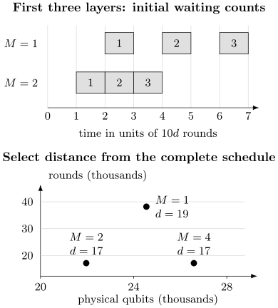
The schedule includes initial production time. One factory leaves gaps between layers; two remove those gaps. After the error budget is imposed, the two-factory design uses both fewer qubits and fewer rounds than the one-factory design. Four factories add qubits without improving this workload’s sequential limit. Numbers follow only from the example’s stated production and error rules.

The physical allocation and runtime are

$$Q=2d^2P(M),\qquad T=\tau_{\mathrm{cyc}}T_{\mathrm{rounds}}.$$

Factories	Physical qubits	Rounds
1	24,548	38,190
2	21,964	17,170
4	26,588	17,170

At $\tau_{\mathrm{cyc}}=1\,\mu\mathrm{s}$, these times are about 38.2 ms, 17.2 ms and 17.2 ms. The exact integer counts are useful for checking the example; they do not make a real fitted noise law exact. If acceptance becomes random or communication delays are introduced, recompute the schedule and exposure.

Physical occupancy, clock time and restarts

A real layout must include work qubits, factories, routing, buffers, input and output regions, and any reserve capacity that is provisioned. The common leading estimate $2d^2$ per surface-code patch is a chosen geometric convention, not a conversion valid for every code. Lattice-surgery layouts make the relation between logical operations and occupied area explicit. For quantum LDPC codes, connectivity, check ancillas and decoding replace the simple planar-patch model.

For time-dependent allocated hardware, distinguish

$$Q_{\mathrm{peak}}=\max_t Q(t)$$

from spacetime volume

$$V_{Qt}=\int_0^T Q(t)\,dt.$$

Constant occupancy gives $V_{Qt}=QT$. If “active” qubits exclude idle but still protected data, that definition undercounts the error exposure. State which occupancy is being integrated.

A code cycle includes the entire syndrome-extraction schedule. Four successive 20 ns gates, a 100 ns measurement, an 80 ns reset and 40 ns synchronization take 300 ns when sequential. The 20 ns gate time is not the cycle time. Overlap can shorten the sum only if dependencies and hardware permit it.

Classical throughput and latency are separate. The decoder must process incoming syndromes fast enough to avoid an accumulating queue. A later conditional operation may also wait for a particular decoded result. A Pauli frame can postpone some physical corrections, but it does not remove every dependency of a non-Clifford operation. Gidney and Ekerå’s factoring estimate explicitly includes reaction time, repeated attempts and a spacetime layout, illustrating why a gate count alone is insufficient.

Expected time is not a high-confidence completion time

If attempts have fixed duration $T_0$, independent success probability $s$, and success can be recognized, the number of attempts until success is geometric:

$$\mathbb E[T_{\mathrm{success}}]=\frac{T_0}{s}.$$

The number of attempts giving at least one success with probability $1-\delta$ is

$$n_\delta= \left\lceil\frac{\ln\delta}{\ln(1-s)}\right\rceil$$

for $0<s<1$. Undetected wrong answers cannot simply be retried “until correct.” They require a verification procedure, repeated statistical inference, or an acceptable residual-error budget. If unsuccessful attempts stop early, use their actual duration distribution.

Acceptance and correctness must also be combined conditionally. If an attempt is accepted with probability $a$ and correct with probability $s_{\mathrm{acc}}$ given acceptance, its accepted-and-correct probability is $a s_{\mathrm{acc}}$. Multiplying two unrelated marginal probabilities would assume independence. Applying an acceptance factor again to a rate already defined per accepted output double-counts the loss.

Sensitivity and useful comparisons

Distance, factory count and module count are discrete. A small parameter change can leave the selected design unchanged, then force a jump. A derivative within one plateau can therefore miss the cost of the next distance. Enumerate supported designs around the boundary and compare feasible alternatives.

Uncertain inputs should be varied in the complete model. Changing cycle time can affect memory exposure in seconds, decoder demand and communication delays; changing physical error may alter both distance and distillation choices. Preserve physical relationships between varied inputs. Independent optimistic choices can describe no realizable machine.

Compare estimates at the same task accuracy, success convention and gate semantics. A smaller qubit count with much longer runtime may be a useful tradeoff, while a smaller count obtained by excluding factories answers a different question. Resource-estimation tools describes reproducible implementations and parameter sweeps; the equations here explain what those tools need to calculate.

Exercises

1. Round a distance correctly

For $N=10^9$, budget $10^{-3}$ and $p_L(d)=0.05(0.08)^{(d+1)/2}$, find the smallest odd distance at least three.

Solution

The required exponent is at least

$$\frac{\ln(5\times10^{10})}{\ln(12.5)} \approx9.75.$$

Thus $d=19$. Direct substitution gives about $5.37\times10^{-4}$, while $d=17$ gives about $6.71\times10^{-3}$ and fails. Both checks matter near an integer boundary.

2. Follow the buffer in the correct order

Supply 120 states at the start of each interval. Compare demands $(1,199)$ and $(199,1)$ from an empty buffer. Assume newly arrived states can be immediately consumed; capacity limits apply to the leftovers retained for the next interval. What leftover capacity lets the first ordering finish both intervals without a stall?

Solution

The first ordering leaves 119 after interval 1, then has $119+120=239$ and leaves 40. Retaining at least 79 after interval 1 is sufficient to meet the second demand, so a capacity of 79 suffices if the extra 40 are discarded. With capacity 78, the second interval has only 198. Reversing the order causes an immediate shortage of 79. If storage must accommodate every arrival before consumption, its required capacity is different; that is why event order was specified.

3. Optimize an error allocation by enumeration

Two classes have $N_m=10^8$, $N_s=10^6$, and $p(d)=10^{-(d+1)/2}$. Their combined cost is $d_m^2+20d_s^2$, with odd distances at least three. Minimize cost subject to $N_mp(d_m)+N_sp(d_s)\leq10^{-3}$.

Solution

The least feasible surgery distance is 19: distance 17 already spends the entire budget on surgery alone. At $d_s=19$, its contribution is $10^{-4}$, requiring $d_m\geq23$; distance 21 would contribute $10^{-3}$. Thus $(d_m,d_s)=(23,19)$ is feasible, with total error $2\times10^{-4}$ and cost $7749$.

Larger surgery distances only raise cost and cannot reduce memory below 23, because memory at distance 21 alone consumes the full budget. Equal distances require 23 and cost $11109$. Equal protection wastes resources for this declared objective.

4. Separate peak allocation from integrated occupancy

Twenty patches are occupied for the first 4 ms and fifty patches for the next 6 ms. Each uses 578 physical qubits. Find peak qubits and qubit-seconds. Compare with peak qubits multiplied by the full runtime.

Solution

Peak allocation is $50(578)=28{,}900$ qubits. The integrated occupancy is

$$578[20(0.004)+50(0.006)] =219.64\ \text{qubit-seconds}.$$

Peak times duration is 289 qubit-seconds, an upper bound here. It includes hardware that is not occupied during the first interval.

5. Recompute the toy design

Verify the selected distances for one and two factories. Does moving from two factories to four reduce runtime, and how does it affect the round-fault bound?

Solution

For one factory and distance 17,

$$34(2010)(17)10^{-10} =1.16178\times10^{-4}.$$

Distance 19 instead gives $1.29846\times10^{-5}$. With two factories, distance 17 gives $38(1010)(17)10^{-10}=6.5246\times10^{-5}$; distance 15 fails. Four factories still take $1010d$ rounds because the layers are sequential, while protecting more allocated patches raises the bound to $7.8982\times10^{-5}$. Extra production capacity is not useful for this schedule.

6. Mean supply does not prevent a delay

Four factories independently accept with probability $0.9$, each delivering two states if accepted. Compute the chance of a shortage when six states are needed in an interval with no stored states.

Solution

Let $K\sim\operatorname{Binomial}(4,0.9)$. A shortage occurs for $K\leq2$, so

$$\begin{aligned} \Pr(K\leq2) &=0.0001+0.0036 +0.0486\\ &=0.0523. \end{aligned}$$

Mean supply $2\mathbb E[K]=7.2$ exceeds demand, but the shortage probability is still 5.23%. Its effect on total runtime depends on buffering and what happens after a shortage.

7. Price a recognizable restart

Each attempt lasts 6 hours and succeeds recognizably with probability $0.8$, independently. Find expected completion time and a reservation sufficient for 99% probability of success.

Solution

The expectation is $6/0.8=7.5$ hours. Failure of all $n$ attempts has probability $0.2^n$. Two attempts give only 96% chance of at least one success; three give 99.2%. An 18-hour reservation therefore suffices in this model. This reasoning would not identify a correct answer if failures were undetectable.

8. Include all stages of a code cycle

Four two-qubit layers each take 20 ns, followed sequentially by 100 ns measurement, 80 ns reset and 40 ns synchronization. Compute the cycle time. How would doubling this time affect the toy example if all error probabilities per round and all round counts stayed fixed?

Solution

The cycle takes $4(20)+100+80+40=300$ ns. Under the stated fixed-per-round assumptions, doubling it doubles wall-clock runtime and qubit-seconds, leaving selected distance, physical qubits and round-fault bound unchanged. If noise instead accumulates at a fixed rate per second, the per-round error changes too; then the entire protection calculation must be repeated.

References

• M. E. Beverland, P. Murali, M. Troyer, K. M. Svore, T. Hoefler, V. Kliuchnikov, G. H. Low, M. Soeken, A. Sundaram and A. Vaschillo, “Assessing requirements to scale to practical quantum advantage,” arXiv:2211.07629 (2022), arXiv.
• A. G. Fowler, M. Mariantoni, J. M. Martinis and A. N. Cleland, “Surface codes: Towards practical large-scale quantum computation,” Physical Review A 86, 032324 (2012), doi:10.1103/PhysRevA.86.032324, arXiv:1208.0928.
• C. Gidney and M. Ekerå, “How to factor 2048 bit RSA integers in 8 hours using 20 million noisy qubits,” Quantum 5, 433 (2021), doi:10.22331/q-2021-04-15-433, arXiv:1905.09749.
• D. Litinski, “A game of surface codes: Large-scale quantum computing with lattice surgery,” Quantum 3, 128 (2019), doi:10.22331/q-2019-03-05-128, arXiv:1808.02892.
• D. Litinski, “Magic state distillation: Not as costly as you think,” Quantum 3, 205 (2019), doi:10.22331/q-2019-12-02-205, arXiv:1905.06903.