Threshold Theorem

The accuracy-threshold theorem explains how a computer built from imperfect components can carry out an arbitrarily long quantum computation reliably. Below a positive noise strength, increasing the amount of error correction suppresses the remaining logical error. For standard concatenated constructions, the extra work per ideal operation grows only as a power of a logarithm of the computation size and required accuracy.

The conclusion depends on a complete fault-tolerant construction and its noise assumptions. It is not a universal percentage to compare with a measured gate fidelity. This page develops the recursive argument, including why errors in the recovery circuit and correlations between neighboring gadgets matter.

Required background. Why quantum error correction is possible supplies the recovery condition; the stabilizer formalism supplies encoded states and syndromes; fault-tolerant gates explains how a circuit contains the spread of faults.

What the accuracy threshold guarantees

An ideal circuit has $L$ locations: gates, preparations, measurements and any other elementary operations used in its description. A physical implementation must also account for noisy waiting, transport, reset and conditional operations. Leaving storage noise out of the location model can invalidate an otherwise careful argument.

Fix an instruction set, a fault-tolerant simulation scheme, an architecture, a noise class and an output error criterion. A threshold theorem establishes a number $p_*>0$ with the following property. For every fixed $p<p_*$, every finite ideal circuit and every target error $0<\varepsilon<1$, a sufficiently protected simulation meets that target. The physical noise strength remains fixed while the encoding scale increases. Aharonov and Ben-Or give a foundational constant-error-rate theorem in their construction.

We use $p_*$ for a proved sufficient bound. It need not equal the largest noise strength $p_{\mathrm{th}}$ at which a particular family actually works. Establishing a lower bound on $p_{\mathrm{th}}$ says nothing decisive about noise above that bound.

For a classical output distribution, an operational target is

$$\frac12\sum_x \left|P_{\mathrm{FT}}(x)-P_{\mathrm{id}}(x)\right| \leq\varepsilon.$$

A quantum output can instead be compared by trace distance after a specified decoding map. A channel guarantee may use half the diamond norm, including an arbitrary reference system. These metrics describe different tasks; use the guarantee actually proved by the selected theorem. An ideal decoder used in a proof is a mathematical comparison map. Delivering a bare, unprotected physical output through a final noisy gate adds an error that more encoding earlier in the circuit need not remove.

Why is the conclusion surprising? For a sequence of memoryless channels with individual half-diamond errors $\delta_\ell$, telescoping gives

$$\frac12\|\widetilde{\mathcal C}-\mathcal C\|_\diamond \leq\sum_{\ell=1}^L\delta_\ell.$$

If every $\delta_\ell\leq\delta$, the sufficient unprotected requirement is $L\delta\leq\varepsilon$. The threshold construction replaces this increasingly stringent component target by a constant component target and a growing protected circuit. A bath with memory needs its own joint-noise analysis; a list of reduced one-gate channels does not by itself justify this telescoping model.

Fault patterns and protected circuit pieces

A fault is a malfunction at a circuit location. An error is damage to the state. One faulty two-qubit gate can create two errors; subsequent ideal gates can spread them further. Code distance alone therefore does not establish a threshold.

Consider a code that corrects up to $t$ errors, with distance at least $2t+1$. Fault-tolerant gadgets must satisfy suitable correctness and error-containment properties when the total incoming error weight and new fault count are at most $t$. For a gate with several input blocks, counting $t$ incoming errors separately in each block is generally too generous: propagation can combine them in one output block. The concrete requirements belong to the gadget construction.

A rectangle, or Rec, replaces an ideal gate by its encoded implementation followed by correction on its output blocks. An extended rectangle, or exRec, also includes correction on its inputs. Preparations and measurements require corresponding endpoint definitions. The extra leading correction makes it possible to reason about damage inherited from earlier operations.

In a simple classification, a level-1 exRec with at most $t$ faults is called good. The construction proves that such a fault pattern gives the intended decoded operation. This statement covers every placement of those faults, with allowed fault actions as specified by the noise model. A pattern classified as bad is outside that guarantee; it need not actually produce a logical error.

One expresses correctness by moving an ideal decoder through a protected operation and replacing that operation by the intended ideal gate. The leading correction, the allowed input states and any truncated endpoints must be retained in this statement. Simply writing an unrestricted channel identity for an entire noisy exRec would conceal those conditions. The detailed exRec correctness and induction lemmas are developed by Aliferis, Gottesman and Preskill.

Why the shared correction matters

The trailing correction of one exRec is the leading correction of the next. Two adjacent exRecs can therefore be classified as bad because of the same small set of physical faults. Their badness probabilities cannot automatically be multiplied, even if elementary faults were independent.

A level-reduction proof resolves these overlaps, for example by assigning shared correction to one retained region and analyzing the appropriately truncated neighboring region. It must then show that a specified collection of effective faulty locations requires sufficiently many underlying faults. This joint statement lets the reduced circuit satisfy the same type of noise bound as the original circuit. Bounding just one gadget’s marginal failure probability is not enough to repeat the argument indefinitely.

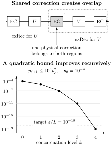
Top: the middle correction belongs to both extended rectangles, so their fault patterns overlap. Bottom: for the illustrative bound $p_{j+1}\leq10^3p_j^2$ with $p_0=10^{-4}$, the plotted upper bounds are $10^{-4},10^{-5},10^{-7},10^{-11},10^{-19}$. With $L=10^{12}$ and $\varepsilon=10^{-6}$, the per-location target is $10^{-18}$; level 4 suffices. These coefficients illustrate the recurrence and do not describe a particular device.

Local noise controls more than single-location errors

For local stochastic noise, let $E$ be the random set of faulty elementary locations. Its strength is bounded by $p$ when

$$\Pr(S\subseteq E)\leq p^{|S|}$$

for every specified set $S$ of locations. Independent faults with individual probabilities at most $p$ satisfy this inequality. Independence is sufficient, but not necessary. Correlations are allowed provided the probability of faults at many specified locations falls sufficiently rapidly.

As a counterexample, suppose a common controller fault damages all $N$ active locations with probability $q$, and otherwise none. Each marginal is $q$, but the probability that any specified $r$ locations are faulty is also $q$, not $q^r$. The smallest admissible local-stochastic parameter for this finite model is

$$p_N=q^{1/N}.$$

It approaches one as $N$ grows. Small marginals therefore do not establish a useful noise bound that is uniform in computer size. This does not mean every correlation destroys fault tolerance; it means this particular parameterization fails for a growing simultaneous burst.

Coherent faults use an amplitude bound

Some threshold theorems allow a shared environment with memory. In a system–environment fault-path expansion, let $F(S)$ be the sum of all paths containing faults at every location in a specified set $S$, with other locations unrestricted. A useful hypothesis has the form

$$\|F(S)\|\leq\eta^{|S|}.$$

The parameter $\eta$ bounds amplitudes in operator norm. It is not a stochastic failure probability or an average gate infidelity. Interference between fault paths changes the counting argument. Terhal and Burkard establish a local non-Markovian threshold theorem; the exRec framework also has a coherent-noise extension.

For suitable bounded local system–bath coupling terms, a dimensionless scale is

$$\eta\sim\frac{t_0}{\hbar} \max_a\|H_{\mathrm{SB},a}\|,$$

where $t_0$ is a gate duration. The locality and norm hypotheses are essential. An unrestricted coupling to many data qubits is not covered merely because its effect on each isolated qubit looks small.

The distinction is visible even for one qubit. For $U_\theta=e^{-i\theta Z/2}$ relative to the identity,

$$\begin{aligned} r_{\mathrm{avg}}&=\frac23\sin^2(\theta/2),\\ \delta_\diamond&=|\sin(\theta/2)|. \end{aligned}$$

At small angle, average infidelity is quadratic in $\theta$, while half-diamond distance is linear. A theorem using one cannot silently substitute the other. Hardware metrics explains their operational meanings.

Leakage, timing and geometry

A persistent leaked qubit can spread damage through many later gates. Leakage-reduction gadgets bound this propagation by replacing or restoring the computational degree of freedom. Their faults and extra locations change the threshold estimate; see Aliferis and Terhal. Heralded loss can be treated as an erasure only to the extent that detection, replacement and the location information actually supplied to the decoder support that model.

The architecture must supply fresh ancillas, adequate parallelism and classical processing consistent with its assumptions. A decoder backlog creates extra waiting locations. A nonlocal gate construction moved to a nearest-neighbor device needs routing and storage errors included. These effects change the physical circuit, not just its final cost estimate.

From fault counting to recursive suppression

Set $s=t+1$. If a gadget with $M$ locations can fail only after at least $s$ faults, a simple local-stochastic bound is

$$p_1\leq {M\choose s}p^s.$$

Every set of at least $s$ faults contains an $s$-element subset; the union bound counts these possible subsets. It deliberately overcounts, since most need not cause failure. A malignant set is a location set whose allowed fault actions can cause an incorrect decoded operation. Refined bounds count such possibilities and control all omitted higher-order patterns.

It is not generally valid to keep only a leading malignant-pair coefficient and discard the remaining terms. If a justified bound is

$$F(x)=\sum_{r=s}^M A_r x^r,$$

then choosing a range $0\leq x\leq p_*$ allows the uniform estimate

$$F(x)\leq A x^s,\qquad A=\sum_{r=s}^M A_r p_*^{r-s}.$$

One must check this chosen range is mapped into itself. After the joint-noise and overlap analysis has established a uniform recurrence, suppose

$$p_{j+1}\leq A p_j^s,\qquad p_0=p.$$

Define $p_*=A^{-1/(s-1)}$, within the recurrence’s valid range. Then $A p_*^{s-1}=1$, so normalization gives

$$\frac{p_{j+1}}{p_*} \leq\left(\frac{p_j}{p_*}\right)^s.$$

Iterating yields

$$p_k\leq p_* \left(\frac{p}{p_*}\right)^{s^k}.$$

For $0<p<p_*$, the base is below one and the exponent grows exponentially with level. Thus the bound falls doubly exponentially. The inequality alone does not show that the actual error increases above $p_*$: a conservative upper bound may simply cease to be informative there.

Choose the scale for a whole computation

For stochastic faults, a union bound over $L$ reduced locations gives

$$P_{\mathrm{fail}}\leq Lp_k.$$

This final union bound does not require independent logical failures. It requires valid bounds on their probabilities. If the unencoded bound already satisfies $Lp\leq\varepsilon$, set $k=0$. Otherwise, a sufficient integer level is

$$k=\left\lceil\log_s \left[\frac{\ln(Lp_*/\varepsilon)} {\ln(p_*/p)}\right]\right\rceil.$$

The case distinction keeps the logarithms well defined. The noise-free case $p=0$ needs no recursion. At fixed $0<p<p_*$,

$$k=O\!\left(\log\log(L/\varepsilon)\right).$$

For the figure’s parameters, $L=10^{12}$ and $\varepsilon=10^{-6}$, level 3 gives only $Lp_3\leq10$, a vacuous probability bound. Level 4 gives $Lp_4\leq10^{-7}$, which meets the target. Bounding a circuit’s failure and bounding one location’s failure are distinct steps.

Why the overhead is polylogarithmic

Suppose one encoding level replaces each location by at most $G$ lower-level locations. The physical count is bounded by $LG^k$. Writing

$$R=\frac{\ln(Lp_*/\varepsilon)}{\ln(p_*/p)},$$

the nontrivial case has $k=\lceil\log_s R\rceil$, hence

$$G^k\leq G R^{\log_s G}.$$

For fixed subthreshold $p$, the denominator is a positive constant. Therefore

$$L_{\mathrm{phys}} =O\!\left(L[\ln(L/\varepsilon)]^{\log_sG}\right).$$

This derivation also identifies what the notation hides. The constant depends on $\ln(p_*/p)$ and can become large near threshold. With $G=100$, the four-level example already has a bound of $10^8$ physical locations per ideal location. Polylogarithmic growth does not guarantee affordable resources.

Depth and qubit counts require their own gadget bounds and scheduling assumptions. Rejected ancilla preparations need a bound on attempts or a high-probability schedule if the claimed cost is not merely an expectation. The required universal operations, including non-Clifford resources, must be included in the construction.

Topological-code arguments instead suppress sufficiently long damaging paths in space and time. Under an applicable bound $p_L(d)\leq C e^{-\alpha d}$ with $\alpha>0$, a sufficient distance is

$$d\geq\frac1\alpha\ln(CL/\varepsilon).$$

Dennis and collaborators develop this connection between fault paths and topological memory. A polynomial prefactor in $d$ changes details but leaves logarithmic distance scaling at fixed noise. Surface codes and lattice surgery explain the resulting area and time costs. Constant space-overhead results require additional assumptions; see quantum LDPC codes.

Thresholds, crossings and finite experiments

A real noise model usually has several rates. A scalar threshold often describes a fixed ray $\boldsymbol p(\lambda)=\lambda\boldsymbol r$ through that parameter space. Changing measurement error relative to gate error, or changing bias, correlations and decoding, changes the ray or the model itself.

Quantity	Question answered
Proved lower bound	Below what strength does this proof guarantee suppression?
Asymptotic threshold	Where does this fixed family cease to suppress error as scale grows?
Finite-size crossing	Where do the tested size-dependent curves intersect?
Pseudothreshold	Where does this encoded operation match its chosen lower-level reference?

A finite experiment showing lower logical error at larger distance tests suppression for the operations and sizes it implements. It does not establish every assumption of a threshold theorem, nor does a protected memory alone establish a universal computation threshold. Logical state preparation, gates, measurement and classical reaction time can introduce other limitations. Logical benchmarking develops those comparisons; resource estimation uses operation-specific error rates to choose a useful scale.

The practical lesson is to retain both parts of a threshold statement: which family becomes more reliable, and under which noise and operational assumptions. Dropping either part turns a useful mathematical result into an ambiguous percentage.

Exercises

1. Find the first sufficient level

Let $p_{j+1}\leq10^3p_j^2$, $p_0=10^{-4}$, $L=10^{12}$ and $\varepsilon=10^{-6}$. Find the first level certified by this bound. What changes if $Lp_0\leq\varepsilon$ already?

Solution

Here $p_*=10^{-3}$ and

$$Lp_k\leq10^{9-2^k}.$$

The target requires $2^k\geq15$, so $k=4$. Level 3 gives the useless upper bound 10; level 4 gives $10^{-7}$. If $Lp_0\leq\varepsilon$, level 0 is sufficient for the stated bound and one should not insert a nonpositive logarithm into the level formula.

2. Keep the higher-order faults

Suppose a valid reduced-noise bound is $F(x)=1000x^2+10^6x^3$. Find its positive intersection with $F(x)=x$. Does retaining only the quadratic term give a rigorous sufficient threshold?

Solution

For $x>0$, the equation becomes

$$10^6x^2+1000x-1=0.$$

The positive solution is

$$p_*=\frac{\sqrt5-1}{2000} \approx6.18\times10^{-4}.$$

For $0<x<p_*$, the full polynomial is smaller than $x$. The truncated estimate would give $10^{-3}$, where the omitted cubic term is not small: $F(10^{-3})=2\times10^{-3}$. It cannot certify that larger interval.

3. Quantify the overhead

For $s=2$ and $G=100$, compute the polylogarithmic overhead exponent. Explain why $k=O(\log\log(L/\varepsilon))$ alone, without its leading coefficient, would not determine that exponent.

Solution

The explicit level choice gives

$$G^k\leq G R^{\log_2G},\qquad \log_2 100\approx6.644.$$

An unspecified constant multiplying $\log\log(L/\varepsilon)$ becomes a power after exponentiation. The explicit recurrence and ceiling bound, rather than the big-$O$ statement alone, determine the exponent. At $k=4$, $100^4=10^8$.

4. Diagnose a growing burst

All $N$ locations fail together with probability $q=10^{-6}$. Find the smallest local-stochastic parameter for $N=2,6,100$, and its large-$N$ limit.

Solution

Every nonempty subset of size $r\leq N$ requires $q\leq p^r$. For $0<p<1$, the strongest condition is $r=N$, giving $p_N=q^{1/N}$. The values are $10^{-3}$, $0.1$ and approximately $0.871$. The limit is one. The qubit marginals stay tiny while the parameter required by this particular theorem becomes unhelpful.

5. Compare coherent and stochastic noise

For $\theta=10^{-3}$, estimate the infidelity and half-diamond distance of $e^{-i\theta Z/2}$. Compare with a stochastic $Z$ flip having the same average infidelity.

Solution

The coherent rotation has

$$\begin{aligned} r_{\mathrm{avg}}&\approx1.67\times10^{-7},\\ \delta_\diamond&\approx5.0\times10^{-4}. \end{aligned}$$

A $Z$ flip with probability $q$ has $r_{\mathrm{avg}}=2q/3$ and $\delta_\diamond=q$. Equal infidelity requires $q=\sin^2(\theta/2)\approx2.5\times10^{-7}$. The half-diamond errors differ by about a factor of 2000. Equal average infidelity does not identify the relevant threshold parameter.

6. A lower bound need not locate the true transition

As a classical example, encode a bit three times, flip its copies independently with probability $p$, and use a perfect majority vote. Derive its exact error map and compare its threshold with the bound obtained by counting all fault pairs. This is an analogy for fault counting, not a quantum fault-tolerant construction.

Solution

Two or three flipped bits give

$$\begin{aligned} f(p)&=3p^2(1-p)+p^3\\ &=3p^2-2p^3. \end{aligned}$$

The nontrivial fixed point is $p=1/2$ and $f(p)<p$ for $0<p<1/2$. Counting all three pairs gives $f(p)\leq3p^2$, which certifies only $p<1/3$. At $p=0.4$, the exact output error is $0.352<p$, although the bound gives $0.48>p$. Exceeding the proved sufficient bound does not imply failure.

7. Convert exponential suppression into a distance

Assume $p_L(d)\leq0.1e^{-d/2}$ per operation. For $10^9$ operations and total target $10^{-3}$, choose a sufficient odd distance. Is independence between logical failures needed here?

Solution

The union bound requires

$$\begin{aligned} e^{-d/2}&\leq10^{-11},\\ d&\geq22\ln10\approx50.66. \end{aligned}$$

Thus $d=51$ suffices under the assumed bound. Independence is unnecessary for the union bound; it may have been needed earlier to establish the individual logical error estimate. Distinguishing those steps avoids transferring an assumption to the wrong part of the argument.

8. Protect the final answer

Suppose a fault-tolerant computation produces its classical answer perfectly, but a final unprotected output wire flips that bit with probability $q>0$. Can increasing the internal code distance guarantee total-variation error below every $\varepsilon>0$?

Solution

For a computation whose ideal output is deterministically 0, the delivered distribution is $(1-q,q)$. Its total-variation distance from $(1,0)$ is exactly $q$. No increase in the earlier code distance removes this final error. A theorem promising arbitrary accuracy must include reliable classical output processing, an appropriately protected classical output, or another explicit output convention. The same issue motivates specifying a decoding map when comparing encoded quantum outputs.

References

• D. Aharonov and M. Ben-Or, “Fault-tolerant quantum computation with constant error rate,” SIAM Journal on Computing 38, 1207–1282 (2008), doi:10.1137/S0097539799359385, arXiv:quant-ph/9906129.
• P. Aliferis, D. Gottesman and J. Preskill, “Quantum accuracy threshold for concatenated distance-3 codes,” Quantum Information and Computation 6, 97–165 (2006), arXiv:quant-ph/0504218.
• P. Aliferis and B. M. Terhal, “Fault-tolerant quantum computation for local leakage faults,” Quantum Information and Computation 7, 139–156 (2007), arXiv:quant-ph/0511065.
• E. Dennis, A. Kitaev, A. Landahl and J. Preskill, “Topological quantum memory,” Journal of Mathematical Physics 43, 4452–4505 (2002), doi:10.1063/1.1499754, arXiv:quant-ph/0110143.
• B. M. Terhal and G. Burkard, “Fault-tolerant quantum computation for local non-Markovian noise,” Physical Review A 71, 012336 (2005), doi:10.1103/PhysRevA.71.012336, arXiv:quant-ph/0402104.