Surface Code

The surface code stores quantum information in extended strings of qubits while measuring local parity checks. Local errors change check outcomes near their endpoints; a classical decoder uses those changes over many rounds to infer a correction. With suitable local noise, a good measurement schedule, and sufficiently accurate operations, larger patches can suppress logical errors.

The central distinction is between the code, which specifies an encoded subspace, and its repeated measurement procedure, which must protect that subspace while the measurements themselves are noisy. We will connect the geometry to a complete nine-qubit patch, then explain error histories, decoding, thresholds, and logical parity measurements. The geometric construction and repeated-measurement analysis are developed by Bravyi and Kitaev and Dennis and colleagues.

Required background. Stabilizer Formalism explains code spaces and Pauli checks. Why Quantum Error Correction Is Possible explains correction without reading the logical state. Syndrome Measurement supplies parity-measurement circuits, and Common Noise Models distinguishes data noise from noisy operations.

Local checks detect the endpoints of error strings

A useful starting picture places a data qubit on each edge of a square lattice. At a vertex v and face p, define

$$A_v=\prod_{e\ni v}X_e, \qquad B_p=\prod_{e\in\partial p}Z_e.$$

The star check $A_v$ compares the adjacent edges in the X basis. The plaquette check $B_p$ compares the edges surrounding a face in the Z basis. A star and a plaquette share zero or two edges, so their X/Z anticommutation signs cancel. The code occupies the common $+1$ eigenspace of the chosen checks.

Now apply Z along a connected path of edges. An interior vertex touches two error edges and still has star eigenvalue $+1$. Each endpoint touches one error edge and has eigenvalue $-1$. Thus the X-check syndrome identifies the endpoints, rather than every edge of the error path. X-error paths have the corresponding description on the dual lattice, whose vertices sit at plaquette centers.

A contractible closed Z path is a product of plaquette checks and has no effect on an encoded state. A noncontractible path can also have no endpoints, yet act as a logical operator. Error correction must distinguish these possibilities using the measured syndrome and the noise model.

On a torus, two independent noncontractible directions encode two logical qubits. On a planar patch, boundaries replace the periodic geometry. In the convention used here:

• A rough boundary allows a Z string to end without a detected endpoint.
• A smooth boundary allows an X string to end without a detected endpoint.

The physical termination rule matters more than the name, since drawings sometimes exchange X and Z. A one-qubit patch has two rough and two smooth boundary segments. A Z string joining distinct rough boundaries and an X string joining distinct smooth boundaries can cross at one data qubit and therefore anticommute. They form a logical Z/X pair.

A complete distance-three rotated patch

Rotated patches use a different boundary layout and a more economical data-qubit arrangement than the unrotated edge-qubit patch. Here is a complete $[[9,1,3]]$ example, with qubits numbered across each row from top to bottom:

$$\begin{matrix} 1&2&3\\ 4&5&6\\ 7&8&9 \end{matrix}.$$

Take all eight listed checks with positive signs:

X checks	Z checks
$X_1X_2X_4X_5$	$Z_1Z_2$
$X_3X_6$	$Z_2Z_3Z_5Z_6$
$X_4X_7$	$Z_4Z_5Z_7Z_8$
$X_5X_6X_8X_9$	$Z_8Z_9$

The bulk checks have weight four and the boundary checks weight two. Every cross-type overlap is even. The eight checks are independent, leaving $2^{9-8}=2$ code states. Convenient logical operators are

$$\overline Z=Z_2Z_5Z_8, \qquad \overline X=X_4X_5X_6.$$

They commute with every check and overlap on qubit 5, giving logical anticommutation. Each has weight three. No Pauli of weight one or two acts as a nontrivial logical operation; Exercise 1 establishes the matching lower bound. Some weight-two Paulis are stabilizers, so this code is degenerate for single-qubit errors.

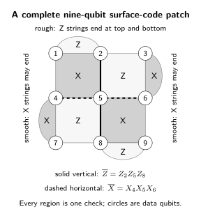
Each square or curved boundary region marks the support of its X or Z check; the numbered circles are data qubits. The vertical logical Z string joins the top and bottom rough boundaries, and the horizontal logical X string joins the left and right smooth boundaries. They share qubit 5. The table specifies every check, including the four boundary checks.

This is an abstract code layout, not a complete measurement circuit. Fowler and colleagues develop surface-code layouts and their implementation through local measurements.

Static distance and circuit distance are different

The static code distance is the minimum weight of a nontrivial logical Pauli, ignoring global phases. It depends on the stabilizer group and boundary layout. A narrow connection or nearby holes can shorten a logical string and reduce that distance.

The circuit distance instead counts elementary faults in a specified preparation, measurement, and readout procedure that can produce an undetected logical failure. It depends on the fault model, gate order, number of rounds, temporal boundaries, and logical observable being tested. A poor extraction schedule can reduce circuit distance while leaving the static stabilizers unchanged.

For the common odd-distance rotated square patch,

$$\begin{aligned} n_{\rm data}&=d^2,\\ n_X=n_Z&=(d^2-1)/2. \end{aligned}$$

With one dedicated ancilla for every check, the patch uses $2d^2-1$ qubits. At $d=5$ this is 25 data qubits and 24 check ancillas. A common unrotated layout instead has $d^2+(d-1)^2$ data qubits. These counts exclude routing, spare qubits, and additional leakage-removal resources.

Repeated measurements separate data errors from readout errors

A single round cannot reliably distinguish a changed data parity from a wrong reported outcome. Measure the checks repeatedly. For a fixed check a with reported sign $m_a(t)$, define

$$\delta_a(t)=m_a(t)m_a(t-1).$$

A value $-1$ is a detection event: the reported check sign changed. This simple definition assumes the same check is expected to persist between rounds. Preparation, final data measurements, changing checks, and known Pauli-frame offsets require the corresponding deterministic parity relations.

Consider one check initially in the $+1$ sector:

Cause	Reported signs at rounds $0,1,2,3,4$	Event rounds
Persistent data error begins before round 2	$+,+,-,-,-$	$2$
Only round 2 is reported incorrectly	$+,+,-,+,+$	$2,3$

In the bulk, a single data error generally changes two neighboring checks, producing two spatially separated events. A single wrong check report produces two temporally separated events at the same check. This turns decoding into a problem in spacetime. Boundaries can absorb one endpoint, and preparation/readout determine which temporal endpoints are allowed.

A hook error from one ancilla fault

To measure a Z check, a common circuit uses data qubits as CNOT controls and the ancilla as target. A Z fault on that ancilla propagates back to each later data control. If it occurs after the second of four interactions, it can leave a two-data Z error called a hook.

For the check $Z_2Z_3Z_5Z_6$, interaction order $(2,5,3,6)$ leaves the pair $Z_3Z_6$ from such a fault. That vertical pair lies along a short logical Z direction: adding $Z_9$ completes the logical string $Z_3Z_6Z_9$. Order $(2,3,5,6)$ instead leaves the horizontal pair $Z_5Z_6$.

This example explains why hook orientation matters. It does not by itself count the circuit distance: other checks measured before and after the fault may reveal additional events. A complete schedule must avoid simultaneous use of a data qubit and must be checked against all allowed fault histories. There is no universally safe clockwise ordering independent of the boundary geometry. Stephens (2014) studies the dependence of fault-tolerant thresholds on circuit choices.

Leakage, correlated control faults, and delayed reset can produce patterns beyond these simple single-Pauli examples. Their effects belong in the noise and measurement model used by the decoder.

A decoder chooses a logical class

With perfect syndrome information, let E be the actual Pauli error and R a correction with the same syndrome. Their product has zero syndrome. Recovery succeeds if $RE$ is a stabilizer up to a global phase; it fails if the product acts as a nontrivial logical Pauli. The decoder need not reproduce the microscopic error exactly.

For the nine-qubit patch, the Z strings on columns 1 and 2 are equivalent:

$$(Z_1Z_4Z_7)(Z_2Z_5Z_8) =(Z_1Z_2)(Z_4Z_5Z_7Z_8).$$

Their difference is a product of two listed checks. By contrast, a single $Z_2$ error and a pair $Z_5Z_8$ have the same syndrome but differ by $\overline Z$. A decoder choosing $Z_2$ succeeds on the first and changes the logical state after the second.

Matching paths between detection events

In an independent graphlike stochastic-fault model, each elementary mechanism produces zero, one, or two detection events, with a single event paired to an allowed boundary. A matching decoder joins the observed events by candidate paths of minimum total weight. For an edge mechanism of probability $p_e<1/2$, a common weight is

$$w_e=\log\frac{1-p_e}{p_e}.$$

These are probability weights, not necessarily geometric lengths. The decoding graph includes spatial, temporal, and schedule-dependent connections. If a fault produces more than two events, its correlations need additional treatment; splitting it into independent edges can change the statistical model.

Even for graphlike noise, the most likely individual error pattern need not belong to the most likely logical class. Many stabilizer-equivalent patterns can contribute to one class, so maximum-likelihood logical decoding sums their probabilities. Separate X and Z matching can also discard correlations associated with Y errors. Decoders develops these distinctions and alternative algorithms.

Corrections are usually tracked in a Pauli frame rather than immediately applied as physical gates. The controller propagates the frame through later Clifford gates and adjusts measurement interpretation. Non-Clifford operations may require adaptive control based on that frame. This avoids unnecessary correction pulses while preserving the intended logical statistics.

Thresholds describe scaling under a specified noise model

A threshold refers to a family of increasing code sizes using a specified noise model, measurement procedure, decoder, and error metric. Below threshold, increasing distance permits asymptotic suppression of logical error. Code-capacity models have perfect check measurements; phenomenological models add faulty outcomes; circuit-level models place faults in the actual operations. Their thresholds need not coincide.

Finite-size improvement, such as $p_L(d+2)<p_L(d)$, demonstrates suppression over the tested distances. It is consistent with below-threshold operation, but a few sizes do not alone establish an asymptotic threshold or validate arbitrarily small extrapolated error rates. A finite-size crossing and an encoded-versus-unencoded pseudothreshold are also different quantities.

An often useful low-noise fit for odd distances is

$$p_L(p,d)\approx A\left(\frac{p}{p_*}\right)^{(d+1)/2}.$$

Here $A$ and $p_*$ are fitted parameters for one stated metric and experiment. The fitted scale $p_*$ is not automatically the asymptotic threshold. The exponent reflects a construction and decoder in which roughly half a distance’s worth of sufficiently independent faults can cause failure. Correlations, reduced circuit distance, or a change of dominant mechanism can invalidate the fit.

The error metric also matters. Logical error per round, final readout error after many rounds, and failure of a logical parity operation are not interchangeable. Exercise 8 shows how even a simple repeated logical-flip model distinguishes them. Dated experiments and their measured performance are discussed in Error-Correction Case Studies.

Lattice surgery measures a joint logical parity

Lattice surgery changes checks along adjacent patch boundaries to measure a joint logical operator, such as $\overline Z_1\overline Z_2$. New checks are repeated, and their outcomes are combined with boundary information to infer a protected parity. A merge joins regions of the code; a split restores separate patches. The geometry and measurement history must preserve the required protection during the change, as developed by Horsman and colleagues.

Joint parity measurement reveals whether two logical Z values agree, without revealing either value separately. For example, a $+1$ outcome preserves coherence between $\lvert0_L0_L\rangle$ and $\lvert1_L1_L\rangle$. This is what allows parity measurements to create entanglement and implement gates.

A logical CNOT can be assembled using an ancilla patch in $\lvert+_L\rangle$, joint ZZ measurement with the control, joint XX measurement with the target, and final Z measurement of the ancilla, followed by outcome-dependent Pauli-frame updates. The full protocol and correction rules are given in Lattice Surgery, rather than being implied by a picture of touching boundaries.

Standard distance-preserving implementations commonly require $O(d)$ syndrome rounds and $O(d^2)$ qubit area, giving $O(d^3)$ qubit-round volume per operation. This describes a common construction, not a universal lower bound on every possible protocol. Preparation, routing, and neighboring operations determine the constants.

From a patch to a protected computation

If N logical locations are assigned error probability at most $\epsilon/N$, the union bound gives total failure probability at most $\epsilon$. Independence is not needed for that bound, though the individual error estimates still need a valid model. Exercise 6 illustrates how a scaling fit turns such an allocation into a candidate distance.

Patch qubit counts are only one part of the resulting machine size. Logical data, routing space, temporary ancillas, and non-Clifford state factories can have very different demands. Measurement time and decoder throughput also matter: a decoder that accumulates an ever-growing backlog cannot support indefinite operation. Resource Estimation connects these costs to a computation.

Finally, active protection should not be confused with passive thermal stability. In the ordinary two-dimensional toric-code Hamiltonian, an error string can grow while carrying only its endpoint excitations; its energy barrier does not grow with string length. Repeated syndrome extraction and decoding supply the active correction. The broader relation between topological encoding and passive memories is developed in Topological Codes.

Exercises

1. Verify the nine-qubit patch

Check commutation and independence of the eight generators. Show that the displayed logical strings have distance three rather than merely weight three.

Solution

Every X/Z overlap in the table has size zero or two. The four supports in each sector are independent by binary row reduction; pure-X and pure-Z generators contribute independently, so the stabilizer rank is eight and the code encodes one qubit.

For pure X, the only weight-two words in the kernel of the Z-check matrix are supports $\{3,6\}$ and $\{4,7\}$, both X stabilizers. For pure Z, the only weight-two words in the X-check kernel are $\{1,2\}$ and $\{8,9\}$, both Z stabilizers. Neither kernel has a weight-one word. A mixed Pauli with total weight at most two has component supports of weight at most two; if it has zero syndrome, both components are stabilizer supports. Its logical action is therefore scalar.

The displayed weight-three X and Z strings commute with all checks and anticommute with one another, so neither is a stabilizer. They attain the lower bound $d=3$.

2. Count logical qubits on a torus

For a connected square cellulation of a torus with V vertices, E edges and F faces, use the check dependencies and Euler relation to count encoded qubits.

Solution

The product of all stars is identity, as each edge appears twice. The same holds for all plaquettes. There is one independent relation in each sector, so the total rank is $V+F-2$. Euler’s relation is $V-E+F=0$, giving

$$k=E-(V+F-2)=2.$$

The two independent noncontractible directions give the corresponding logical cycles. Open planar boundaries change this count and must be specified separately.

3. Compare three recoveries

Why are Z strings on the first and second columns equivalent logical operators? Why does choosing correction $Z_2$ fail after error $Z_5Z_8$ even though the syndrome is removed?

Solution

The product of the two columns is $(Z_1Z_2)(Z_4Z_5Z_7Z_8)$, a product of Z checks. They therefore have the same action on every code state. But $Z_2Z_5Z_8=\overline Z$ is a logical operator. The actual pair $Z_5Z_8$ has the same syndrome as $Z_2$, and the chosen correction returns the data to the code space while applying logical Z. Zero residual syndrome alone does not establish successful recovery.

4. Find detection events in time

For one check, compare the sign records $(+,+,-,-,-)$ and $(+,+,-,+,+)$ at rounds 0 through 4. Identify the event times and the physical interpretation under the simple noise models in the text.

Solution

Multiplying neighboring signs gives $\delta(1),\ldots,\delta(4)=(+,-,+,+)$ for the first record and $(+,-,-,+)$ for the second. A persistent data change before round 2 gives an event at round 2. A wrong report only at round 2 gives events at rounds 2 and 3. Initial and final boundaries need additional known parity relations; these interior comparisons alone do not define a complete memory experiment.

5. Propagate an ancilla Z fault

In a Z-check circuit with data controls and ancilla target, insert ancilla Z immediately after the second CNOT. Determine the final data error for orders $(2,5,3,6)$ and $(2,3,5,6)$. Does this calculation alone establish circuit distance?

Solution

CNOT conjugates target Z to control Z times target Z. The fault therefore adds Z to each remaining data control, leaving $Z_3Z_6$ for the first order and $Z_5Z_6$ for the second. Ancilla Z does not itself flip the final Z readout.

The first pair can be extended by $Z_9$ to the weight-three logical column $Z_3Z_6Z_9$. However, checks elsewhere in the global schedule may record changes before or after the fault. A circuit-distance claim must compare the entire observable and detector history under the declared fault model, not only the final data Pauli.

6. Choose a distance from an illustrative fit

Suppose a per-cycle fit gives $A=0.1$ and $p/p_*=0.1$. Allocate failure probability $0.01$ across $10^8$ logical patch cycles. What smallest odd distance meets this allocation according to the fit, and how many qubits are in one idealized rotated patch with one ancilla per check?

Solution

The per-cycle allocation is $10^{-10}$. The fit gives

$$p_L=10^{-1-(d+1)/2}.$$

Hence $(d+1)/2\ge9$, so the smallest odd distance is $d=17$. Distance 15 predicts $10^{-9}$ and fails the allocation. At distance 17 the idealized patch has 289 data qubits, 288 check ancillas, and 577 total qubits.

This is a conditional model prediction. It requires the fitted per-cycle behavior to remain valid at the selected distance, and it does not include other patch resources or logical-operation errors. The symbol $p_*$ need not be an independently established threshold.

7. Create entanglement by measuring parity

Start with two logical qubits in $\lvert+_L+_L\rangle$. Find the probabilities and normalized states after measuring $\overline Z_1\overline Z_2$.

Solution

The initial state has amplitude $1/2$ on each logical computational pair. The even and odd projectors each retain two terms and therefore each have probability $1/2$. Their normalized outputs are

$$\begin{aligned} \lvert\Phi_+\rangle&=\frac{\lvert00\rangle_L+\lvert11\rangle_L}{\sqrt2},\\ \lvert\Psi_+\rangle&=\frac{\lvert01\rangle_L+\lvert10\rangle_L}{\sqrt2}. \end{aligned}$$

Each outcome preserves coherence within its parity sector and produces an entangled state. Measuring the two logical Z values separately would instead reveal the individual bit pair and remove that coherence.

8. Distinguish final parity from any failure

Suppose independent logical flips occur with probability q per round. After T rounds, find the probability of an incorrect final parity and the probability that at least one flip occurred.

Solution

Final parity is wrong after an odd number of flips. The even-minus-odd probability is $(1-2q)^T$, so

$$p_{\rm odd}=\frac{1-(1-2q)^T}{2}.$$

The probability of at least one flip is $1-(1-q)^T$. Both approach $Tq$ when $Tq\ll1$, but they differ when multiple flips become appreciable. At $q=0.1,T=2$, the probabilities are 0.18 and 0.19. This simple model illustrates why final readout error and an accumulated failure metric are different; real logical channels may contain more than one type of error or time correlations.

References

• S. B. Bravyi and A. Y. Kitaev, “Quantum codes on a lattice with boundary,” 1998, arXiv:quant-ph/9811052.
• E. Dennis, A. Kitaev, A. Landahl, and J. Preskill, “Topological quantum memory,” Journal of Mathematical Physics 43, 4452–4505, 2002, doi:10.1063/1.1499754, arXiv:quant-ph/0110143.
• A. G. Fowler, M. Mariantoni, J. M. Martinis, and A. N. Cleland, “Surface codes: Towards practical large-scale quantum computation,” Physical Review A 86, 032324, 2012, doi:10.1103/PhysRevA.86.032324.
• D. Horsman, A. G. Fowler, S. Devitt, and R. Van Meter, “Surface code quantum computing by lattice surgery,” New Journal of Physics 14, 123011, 2012, doi:10.1088/1367-2630/14/12/123011.
• A. M. Stephens, “Fault-tolerant thresholds for quantum error correction with the surface code,” Physical Review A 89, 022321, 2014, doi:10.1103/PhysRevA.89.022321.