GKP Codes

A Gottesman–Kitaev–Preskill (GKP) code stores a qubit in an oscillator using a periodic grid in phase space. Small shifts of position and momentum can be measured modulo a lattice spacing without reading out the logical state. Correcting the measured residue leaves a discrete logical Pauli error only when the decoder chooses the wrong lattice class.

The ideal code makes this geometry exact but has infinite energy. Physical grid states have finite peaks and an envelope, and their recovery adds noise. We will first derive the ideal qubit, then calculate its displacement errors and analog likelihoods, before explaining what changes at finite energy and during gates.

Required background. Bosonic Codes introduces oscillator encodings and recovery. Stabilizer Formalism explains commuting checks and logical operators. Coherent States in Phase Space supplies displacement operators, while Continuous-Variable Systems develops quadratures and Gaussian transformations.

Commuting translations define the square GKP qubit

Use dimensionless quadratures with vacuum variance $1/2$:

$$\begin{aligned} q&=(a+a^\dagger)/\sqrt2,\\ p&=(a-a^\dagger)/(i\sqrt2),\\ [q,p]&=i,\qquad n=(q^2+p^2-1)/2. \end{aligned}$$

A displacement $W(u,v)=e^{i(vq-up)}$ shifts the means of $q,p$ by $u,v$. With vectors $\xi=(u,v)$ and $\xi'=(u',v')$, define their signed area $\xi\wedge\xi'=uv'-vu'$. The Weyl relation is

$$W(\xi)W(\xi') =e^{-i\xi\wedge\xi'/2}W(\xi+\xi').$$

Reversing the order changes the phase by $e^{-i\xi\wedge\xi'}$. Thus translations commute when the enclosed area is an integer multiple of $2\pi$. This allows two commuting modular checks even though $q$ and $p$ themselves do not commute.

Write $b=\sqrt\pi$. The square qubit has stabilizers

$$\begin{aligned} S_Z&=e^{2ibq}=W(0,2b),\\ S_X&=e^{-2ibp}=W(2b,0). \end{aligned}$$

Their area is $4\pi$, so they commute. The code is their simultaneous generalized $+1$ eigenspace. In position space,

$$\langle q|\mu_L\rangle\propto \sum_{s\in\mathbb Z}\delta\bigl(q-(2s+\mu)b\bigr),$$

where $\mu=0,1$. Logical zero occupies even sites and logical one odd sites. The momentum-space combs of $|+_L\rangle$ and $|-_L\rangle$ have the corresponding even and odd structure. These are distributions, not normalizable oscillator vectors. Their exact translation symmetry is a mathematical reference for finite-energy states, as in the original construction of Gottesman, Kitaev, and Preskill (2001).

Half translations give the logical Paulis:

$$Z_L=e^{ibq},\qquad X_L=e^{-ibp}.$$

$Z_L$ multiplies a position-comb site by $(-1)^\mu$, while $X_L$ exchanges even and odd sites. They commute with the stabilizers and anticommute with each other because their enclosed area is $\pi$. Their squares are stabilizers. The stabilizer length is $2b$; the logical translation length is $b$. Neither is the half-cell correction radius $b/2$.

Conventions using $[q,p]=i/2$ or the complex amplitude $\alpha=(u+iv)/\sqrt2$ assign different numerical lengths to the same geometry. Quadrature normalization must accompany any quoted spacing or squeezing.

Modular syndromes and residual logical errors

After an error $W(u,v)$, the stabilizer eigenvalues become

$$S_Z:\ e^{2ibu},\qquad S_X:\ e^{-2ibv}.$$

These phases reveal $u,v$ modulo $b$. They do not reveal whether the logical comb occupied even or odd sites. Choose centered residues $r_q,r_p\in[-b/2,b/2)$ and apply $W(-r_q,-r_p)$. The remaining translation, up to overall phase, is

$$W(mb,nb),\qquad m,n\in\mathbb Z.$$

Its logical action depends only on the parities of those integers:

$m$ parity	$n$ parity	Residual Pauli
Even	Even	$I$
Odd	Even	$X$
Even	Odd	$Z$
Odd	Odd	$Y$, up to phase

Every shift strictly inside the centered square is corrected by this ideal procedure. Shifts outside it can also be harmless: a remaining translation by $2b$ is a stabilizer. A boundary is ambiguous for a symmetric prior, and a different prior or further measurements may change the preferred correction.

For instance, $(u,v)=(0.63,-0.18)b$ has residue $(-0.37,-0.18)b$. Canceling that residue leaves $(b,0)$ and hence logical $X$. The syndrome can be measured perfectly while the recovery still makes a logical error.

Stabilizer lattice and commuting displacement lattice

The stabilizer lattice is $\Lambda_S=2b\mathbb Z^2$. All displacements commuting with it form the symplectic dual $\Lambda_S^\perp=b\mathbb Z^2$. Their quotient has four classes, corresponding to $I,X,Z,Y$. This lattice description generalizes to multiple modes; Conrad, Eisert, and Arzani (2022) develop the construction.

The shortest nontrivial logical translation has Euclidean length $b$. This displacement distance is not a qubit Hamming weight. For isotropic Gaussian shifts, the centered square is the nearest-lattice cell. Anisotropic or correlated noise changes the relevant likelihood metric, and more general lattices have different correction cells.

Gaussian errors and the value of an analog outcome

Assume, for this section only, an ideal code and ideal syndrome measurement with a classical Gaussian displacement prior. If the position shift has mean zero and variance $\sigma^2$, write its density as $f_\sigma(u)$. Nearest-lattice correction leaves odd position parity with probability

$$p_q=\sum_{\substack{m\in\mathbb Z\\m\ {\rm odd}}} \int_{(m-1/2)b}^{(m+1/2)b} f_\sigma(u)\,du.$$

For a narrow distribution, the nearest wrong cells dominate:

$$p_q\simeq\operatorname{erfc} \!\left(\frac{b}{2\sqrt2\sigma}\right).$$

The complementary-error-function expression counts all probability outside the central interval. It is an upper bound on the exact odd-cell sum, with excellent agreement when farther cells are negligible. At larger noise it includes even cells that yield stabilizers and must not be treated as the exact logical error probability.

$\sigma/b$	Exact $p_q$	Central-interval tail
0.2	0.01242	0.01242
0.4	0.21112	0.21130
0.8	0.47294	0.53197

For independent position and momentum shifts, with odd probabilities $p_q,p_p$, the resulting Pauli probabilities are

$$\begin{aligned} P_I&=(1-p_q)(1-p_p),\\ P_X&=p_q(1-p_p),\\ P_Z&=(1-p_q)p_p,\\ P_Y&=p_qp_p. \end{aligned}$$

Thus $p_q$ is the probability of an $X$ component, including $Y$, rather than the probability of an exclusively $X$ error. This distinction matters when combining the two quadratures.

Sum all compatible shifts in each logical class

A measured residue $r$ is compatible with every shift $r+kb$. Bayes’ rule gives the unnormalized class likelihoods

$$L_j(r)=\sum_{k\equiv j\;({\rm mod}\;2)} \exp\!\left[-\frac{(r+kb)^2}{2\sigma^2}\right],$$

for $j=0,1$. The conditional odd probability is $L_1/(L_0+L_1)$, and the log-likelihood ratio is $\log(L_0/L_1)$. A residue near zero strongly favors an even hidden index under a narrow prior; near $b/2$ the two classes compete. Fukui, Tomita, and Okamoto (2017) show how retaining analog information can improve decoding beyond a hard binary decision.

For $\sigma=0.2b$, residues $0.05b$ and $0.49b$ have conditional odd probabilities about $1.41\times10^{-5}$ and $0.438$. The same nearest-cell decision therefore carries very different confidence.

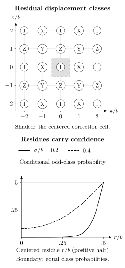
Top: lattice points represent residual translations, labeled by their logical Pauli class. The central shaded square is the nearest-lattice correction cell. This is displacement space, not a Wigner function. Bottom: exact odd-class likelihoods retain how close a residue is to an ambiguous boundary; the prior width changes that confidence.

Closest-point decoding and most-likely-class decoding are different problems. A closest-point decoder selects the single most likely displacement under an isotropic Gaussian prior. A class decoder sums over every displacement differing by a stabilizer before comparing logical outcomes. Closest-point decoding is often a useful small-noise approximation for general multimode GKP codes, but is not the general maximum-likelihood rule. Lin, Chamberland, and Noh (2023) explicitly make this distinction in their lattice-decoding analysis.

With noisy extraction, a decoder must also model ancilla shifts, correlations, and the history of repeated outcomes. Decoders explains the broader use of logical-class likelihoods. The simple Gaussian formulas above do not automatically describe coherent finite-energy effects or a full gate circuit.

Finite peaks, finite envelopes, and physical encoding

A useful finite-energy position wavefunction is

$$\psi_\mu(q)\propto\sum_s e^{-(q-q_{s\mu})^2/(4\sigma^2)} \times e^{-\kappa^2 q_{s\mu}^2/2},$$

with $q_{s\mu}=(2s+\mu)b$. Each isolated peak has probability variance $\sigma^2$ when overlaps are negligible. The envelope scale is set by $\kappa^{-1}$; it controls how many distant peaks contribute. Narrowing peaks without a finite envelope does not yield a normalizable state. Fourier transformation relates the envelope in one quadrature to the peak structure in the other.

Another common regularization is $e^{-\Delta^2 n}|\mu_L\rangle$, followed by normalization. It yields normalizable states for $\Delta>0$ and approaches the ideal comb only as the energy diverges. Royer, Singh, and Girvin (2020) treat finite-energy stabilization directly. Different regularizations need not assign the same numerical width or envelope to a quoted squeezing value.

Two separately normalized states need not be a qubit basis

Finite-width versions of the even and odd combs generally overlap. Simply mapping $u|0\rangle+v|1\rangle$ to $u|\psi_0\rangle+v|\psi_1\rangle$ is then not an isometric encoding: its norm depends on the logical amplitudes. It is not valid to repair this by renormalizing each unknown input, which would make the map nonlinear.

One possible mathematical encoding uses the two columns of $F=(|\psi_0\rangle,|\psi_1\rangle)$ and their positive Gram matrix $G=F^\dagger F$:

$$V=FG^{-1/2},\qquad V^\dagger V=I.$$

This preserves their two-dimensional span and defines an orthonormal logical basis. It is a choice of encoding, not an assertion that experimental preparation automatically implements that map. Alternatively, a stabilizer-subsystem description separates logical information from continuous syndrome degrees of freedom; Shaw, Doherty, and Grimsmo (2024) connect such a decomposition to ideal decoding.

Finite energy changes intrinsic syndrome distributions, state overlap, the action of logical displacements, and gate-induced envelope deformation. A pure broadened comb is not exactly the same state as an ideal comb subjected to classical random displacements. Treating finite preparation noise as independent Gaussian shifts can be useful, but it is a modeling approximation.

Squeezing and recovery noise

With the isolated-peak convention above, one definition is

$$s_{\rm GKP}=-10\log_{10}(2\sigma^2)\ {\rm dB}.$$

It gives $10$ dB for $\sigma^2=0.05$. Stabilizer-based width estimates and optical input squeezing need not be equal to this number. The envelope and quadrature convention are needed to interpret it.

GKP-ancilla extraction uses Gaussian couplings and homodyne outcomes; two-level-ancilla methods use controlled displacements and readout. Teleportation can move the logical state into a fresh prepared mode while extracting syndromes. Dissipative or reset-based stabilization can remove entropy without recording a classical outcome each round. In each case, finite ancilla quality, backaction and control faults contribute to the logical channel. See Bosonic Qubits for physical implementations.

Loss, amplification, and rotations

Pure loss with transmissivity $0<\eta\le1$ sends

$$q\mapsto\sqrt\eta\,q+\sqrt{1-\eta}\,q_e,$$

with a vacuum environment of variance $1/2$, and similarly for $p$. It contracts the grid as well as adding noise. It is not simply a random displacement of the original lattice.

A quantum-limited phase-insensitive amplifier of gain $g=1/\eta$ restores the mean scale. The order matters:

Physical order	Added variance per quadrature
Loss, then amplification	$(1-\eta)/\eta$
Amplification, then loss	$1-\eta$

These composite channels are exactly additive Gaussian displacement channels under the stated vacuum and quantum-limited assumptions, for arbitrary input states, including finite-energy grids. The amplifier adds physical noise; it is not a noiseless inverse of loss. Pre-amplification raises the transmitted energy, and is unavailable if the loss has already occurred. Noh, Albert, and Jiang (2019) analyze these channel decompositions.

Number dephasing instead produces random rotations $e^{-i\theta n}$. A point at radius $r$ moves a distance $2r|\sin(\theta/2)|\simeq r|\theta|$. Distant peaks are therefore more sensitive to the same small angle. Increasing energy can narrow intrinsic grid peaks while increasing exposure to other noise mechanisms. There is no single displacement variance that exactly represents every combination of loss, rotations and ancilla faults.

Gates and other lattice shapes

Suitable Gaussian transformations implement ideal logical Clifford gates. A quarter rotation implements Hadamard up to convention; the shear $(q,p)\mapsto(q,p+q)$ implements a phase gate; and $e^{-iq_1p_2}$ implements SUM, with

$$q_2\mapsto q_2+q_1,\qquad p_1\mapsto p_1-p_2.$$

These transformations preserve the appropriate ideal stabilizer algebra, including phases. An arbitrary Gaussian transformation need not preserve a chosen code: generic squeezing changes its lattice shape. Even a valid ideal Clifford can deform a finite envelope or correlate displacement errors. SUM, for instance, copies a control position shift into the target and a target momentum shift into the control. Correcting both outputs as if their errors were independent discards that correlation.

Universality requires a non-Clifford resource, such as logical magic-state injection or suitable nonlinear control. A projected gate acting correctly on an ideal code is insufficient to establish a protected operation on finite-energy states. Bosonic and Encoded Computation Models explains how the complete physical program determines the recovered logical channel.

A rectangular lattice trades position and momentum correction widths at fixed cell area. A hexagonal lattice has a larger Euclidean packing radius than a square at fixed area, which can help isotropic displacement correction; preparation and gate noise can alter the comparison. Multimode lattices and concatenation with a Surface Code use additional modes and joint decoding to suppress residual logical errors.

For a square logical qudit of dimension $d$, the stabilizer and logical spacings are

$$\ell_d=\sqrt{2\pi d},\qquad \lambda_d=\sqrt{2\pi/d}.$$

Define $Z_d=e^{i\lambda_d q}$ and $X_d=e^{-i\lambda_d p}$. The position comb is $q=(sd+\mu)\lambda_d$, with $\mu=0,\ldots,d-1$, and $Z_dX_d=e^{2\pi i/d}X_dZ_d$. Increasing $d$ increases the stabilizer cell area but decreases the logical spacing. One mode encoding a larger logical system does not supply independently controlled physical modes. Thresholds for concatenated architectures depend on their finite-energy states, extraction circuits, loss, gates and decoder; they are not constants specified by the one-mode lattice alone.

Exercises

1. Check the area and the comb phases

Verify stabilizer commutation and logical anticommutation. Show how $e^{ibq}$ acts on both position combs.

Solution

Stabilizer vectors $(2b,0)$ and $(0,2b)$ enclose $4b^2=4\pi$, giving commutation phase one. Half vectors enclose $b^2=\pi$, giving phase minus one. On $q=(2s+\mu)b$, the phase of $e^{ibq}$ is $e^{i\pi(2s+\mu)}=(-1)^\mu$. Translation by $b$ exchanges the two site parities. These are the Pauli actions without treating the Dirac comb as a normalized state.

2. Decode small and large shifts

Decode $(u,v)=(0.20,-0.41)b$, $(0.72,0.61)b$, and $(2.20,-0.41)b$ by centered residues.

Solution

The first residue is the shift itself, leaving $I$. The second residue is $(-0.28,-0.39)b$, leaving $W(b,b)$, or $Y$ up to phase. The third has the same residue as the first but leaves $W(2b,0)=S_X$, which also acts as identity. Crossing the central cell boundary is therefore not identical to a logical error for every possible shift.

3. Separate a one-axis error from a Pauli probability

For independent equal Gaussian shifts with $\sigma=0.4b$, use $p_q=p_p\simeq0.21112$ to calculate $P_I,P_X,P_Z,P_Y$. Why is the central tail only an approximation to $p_q$?

Solution

The probabilities are approximately $P_I=0.6223$, $P_X=P_Z=0.1665$, and $P_Y=0.0446$. Their sum is one. The position odd probability includes both $X$ and $Y$. The central tail also counts far even cells, although their net translations are stabilizers. As $\sigma/b$ grows without bound, each one-axis parity becomes equally likely and the four Pauli probabilities tend to $1/4$; the central tail instead tends to one.

4. Use all hypotheses behind an analog result

At $\sigma=0.2b$ and $r=0.49b$, estimate the odd-class probability from the two dominant hypotheses. Explain what changes in the full class sum.

Solution

The dominant even shift is $0.49b$, and the dominant odd shift is $-0.51b$. Their log-likelihood ratio is

$$\begin{aligned} \log(L_0/L_1)&\simeq \frac{0.51^2-0.49^2}{2(0.2)^2}\\ &=0.25. \end{aligned}$$

Thus the odd probability is $1/(1+e^{0.25})\simeq0.438$. The full expression adds every even or odd lattice alias; these additions are tiny here, but need not be negligible for broad noise or higher-dimensional lattices. A toy syndrome with one identity-class candidate of probability $0.4$ and two equivalent $X$ candidates of probabilities $0.3$ each would favor $X$ by class probability despite favoring identity by its single largest candidate.

5. Normalize an encoding, not each unknown input

Suppose two normalized approximate grid states have real overlap $\epsilon\ne0$. Find the squared norm of their equal superposition and verify the Gram-matrix encoding.

Solution

The nominal state $(|\psi_0\rangle+|\psi_1\rangle)/\sqrt2$ has squared norm $1+\epsilon$, while the relative-minus state has norm squared $1-\epsilon$. Separate normalization of the two basis columns is therefore insufficient. When they are linearly independent, $G$ is positive definite and

$$V^\dagger V=G^{-1/2}GG^{-1/2}=I.$$

This one linear map preserves the norm and inner product of every logical input. Input-dependent renormalization does not define a deterministic quantum encoding channel.

6. Derive both amplifier-order variances

Use the covariance maps $V\mapsto\eta V+(1-\eta)I/2$ for loss and $V\mapsto gV+(g-1)I/2$ for a quantum-limited amplifier. Set $g=1/\eta$ and compare the two orders at $\eta=0.8$.

Solution

Loss followed by amplification gives two equal vacuum contributions, each $(1-\eta)/(2\eta)$, for total variance $0.25$ per quadrature. Amplification followed by loss gives contributions $\eta(g-1)/2$ and $(1-\eta)/2$, for total $0.20$. Both maps restore unit gain on the input covariance and mean, but their added noises differ. Before transmission, the amplifier changes the mean occupation to $g\bar n+(g-1)$, so the smaller-noise ordering has an energy cost.

7. Follow correlations through SUM

Let the four input shift variables $(u_1,v_1,u_2,v_2)$ be independent, each of variance $s^2$. Find their output variances and the nonzero cross-mode covariances after SUM.

Solution

The output shifts are

$$(u_1,\ v_1-v_2,\ u_2+u_1,\ v_2).$$

Their variances are $(s^2,2s^2,2s^2,s^2)$. The cross-mode covariances are $\operatorname{Cov}(u_1',u_2')=s^2$ and $\operatorname{Cov}(v_1',v_2')=-s^2$; all other cross-mode pairs have zero covariance. Thus an ideal Gaussian gate preserves the code algebra while creating correlations relevant to decoding.

8. Count a square qudit’s lattice cells

Show that $\ell_d=d\lambda_d$, derive the generalized Pauli phase, and compare $d=2$ with $d=4$.

Solution

The ratio is $\ell_d/\lambda_d=d$. Logical translations enclose area $\lambda_d^2=2\pi/d$, so their Weyl relation gives $Z_dX_d=e^{2\pi i/d}X_dZ_d$. For $d=2$, the spacings are $2\sqrt\pi$ and $\sqrt\pi$; for $d=4$, they are $\sqrt{8\pi}$ and $\sqrt{\pi/2}$. There are $d^2$ logical displacement classes modulo stabilizers, corresponding to $X_d^mZ_d^n$ with exponents modulo $d$. The reduced logical spacing means less tolerance to a fixed quadrature shift under nearest-lattice decoding.

References

• J. Conrad, J. Eisert, and F. Arzani, “Gottesman–Kitaev–Preskill codes: A lattice perspective,” Quantum 6, 648 (2022), doi:10.22331/q-2022-02-10-648, arXiv:2109.14645.
• K. Fukui, A. Tomita, and A. Okamoto, “Analog quantum error correction with encoding a qubit into an oscillator,” Physical Review Letters 119, 180507 (2017), doi:10.1103/PhysRevLett.119.180507, arXiv:1706.03011.
• D. Gottesman, A. Kitaev, and J. Preskill, “Encoding a qubit in an oscillator,” Physical Review A 64, 012310 (2001), doi:10.1103/PhysRevA.64.012310, arXiv:quant-ph/0008040.
• M. Lin, C. Chamberland, and K. Noh, “Closest lattice point decoding for multimode Gottesman–Kitaev–Preskill codes,” PRX Quantum 4, 040334 (2023), doi:10.1103/PRXQuantum.4.040334, arXiv:2303.04702.
• K. Noh, V. V. Albert, and L. Jiang, “Quantum capacity bounds of Gaussian thermal loss channels and achievable rates with Gottesman–Kitaev–Preskill codes,” IEEE Transactions on Information Theory 65, 2563–2582 (2019), doi:10.1109/TIT.2018.2873764, arXiv:1801.07271.
• B. Royer, S. Singh, and S. M. Girvin, “Stabilization of finite-energy Gottesman–Kitaev–Preskill states,” Physical Review Letters 125, 260509 (2020), doi:10.1103/PhysRevLett.125.260509, arXiv:2009.07941.
• M. H. Shaw, A. C. Doherty, and A. L. Grimsmo, “Stabilizer subsystem decompositions for single- and multimode Gottesman–Kitaev–Preskill codes,” PRX Quantum 5, 010331 (2024), doi:10.1103/PRXQuantum.5.010331, arXiv:2210.14919.

Further reading

A. L. Grimsmo and S. Puri, “Quantum error correction with the Gottesman–Kitaev–Preskill code,” PRX Quantum 2, 020101 (2021), doi:10.1103/PRXQuantum.2.020101, arXiv:2106.12989, connects the code geometry to preparation and fault-tolerant architectures.