

Decoders
A quantum error-correction decoder uses measured checks and a noise model to choose a recovery. It usually cannot determine the microscopic fault uniquely, and it does not need to. Errors differing by a stabilizer act identically on the code; errors differing by a logical operator can produce the same syndrome but require different recoveries.
The central task is therefore inference about logical classes. We will distinguish that task from finding a single likely error, explain how noisy measurement histories enter, and compare matching, message passing and class-summing methods. A decoder must also return useful decisions on the timescale required by the computation.
Required background. Why Quantum Error Correction Is Possible explains recovery conditions; Stabilizer Formalism defines syndromes and logical Paulis. Syndrome Measurement develops repeated outcomes and detector boundaries, while Surface Code supplies a geometric example.
Decoding is logical-class inference
Section titled “Decoding is logical-class inference”First assume a stabilizer code, stochastic Pauli errors, and an exactly measured syndrome . Let be the stabilizer group. Choose a reference Pauli with that syndrome. Every compatible Pauli has, up to overall phase, the form
where is a representative logical Pauli. An code has such logical classes for each syndrome. The syndrome fixes the commutation signs with checks, but not the logical label .
The class weight is
Normalize by to obtain the posterior probability of each class. Choosing the largest class weight maximizes the chance of a successful Pauli recovery under this model. If is the chosen representative, applying succeeds when is a stabilizer, up to phase.
This is often called maximum-likelihood logical decoding. More precisely, it maximizes a posterior incorporating the assumed fault prior. It differs from choosing the single most probable physical error. Bravyi, Suchara, and Vargo (2014) develop class-based decoding algorithms for surface codes.
A concrete degeneracy example
Section titled “A concrete degeneracy example”Consider the two-qubit code spanned by , with check and logical . It is an illustrative inference problem, not a code correcting arbitrary one-qubit faults. Suppose a Pauli channel assigns the following probabilities, with the remaining probability assigned to identity:
| Error | Probability | Odd-syndrome class |
|---|---|---|
| 0.30 | A | |
| 0.01 | A | |
| 0.20 | B | |
| 0.20 | B |
Within each class, the two errors differ by the stabilizer up to phase. Between classes they differ by logical . The most probable individual error is , but class B has total probability , exceeding class A’s . Conditional on the odd syndrome, correcting class B succeeds with probability , whereas correcting A succeeds with .
Reconstructing the physical error more accurately is not always the same as protecting the logical state more accurately. The sum over stabilizer-equivalent alternatives is the useful feature of quantum degeneracy.
Nonuniform noise can favor a heavier error
Section titled “Nonuniform noise can favor a heavier error”For the Three-Qubit Code with checks , restrict the channel to independent bit flips of probabilities . Syndrome permits exactly two bit patterns: and . Their probabilities are
Equal probabilities favor the weight-one explanation. But if qubit 1 is much cleaner than the other two, the weight-two explanation can win. Minimum Hamming weight is justified by a particular prior; it is not the definition of decoding.
Noisy records require histories of faults
Section titled “Noisy records require histories of faults”With imperfect measurements, the observed bits need not equal the true data-error syndrome. It is then incorrect to restrict inference to data errors having that observed syndrome as though it were exact.
Instead, let label a complete modeled history, including data faults and measurement faults. Let be the observed record, and let denote the logical effect relative to a fixed reference correction and final logical readout convention. The posterior is
An exact observation imposes a hard constraint on this sum; a noisy observation supplies a likelihood. The model must specify which preparation, intermediate and final measurements are available. An offline decoder seeing the final boundary has more information than a streaming decoder asked to decide earlier.
Repeated checks are often converted to detectors: parities of measurement outcomes that are deterministic without faults. In a simple bulk region,
A wrong readout bit usually creates two adjacent time changes; a persistent data error can change the underlying syndrome. Initial and terminal detectors require their own boundary definitions. The derivation belongs to the extraction circuit, rather than to a generic difference formula applied everywhere.
For binary elementary faults collected in a vector , a detector model can be written
over . Each column specifies the detectors and tracked logical observables flipped by one mechanism. Two histories can have identical and different , which is precisely the ambiguity the decoder must resolve. Independent Bernoulli faults are one convenient model; mutually exclusive Pauli outcomes, bursts and persistent leakage need more care.
Hard and soft information
Section titled “Hard and soft information”A hard decoder receives thresholded bits. A soft decoder also uses reliability information, such as analog voltages, erasure flags or GKP residues. Suppose a readout value has distributions and . Its likelihood ratio is
The posterior log odds also include the prior log odds of the two hypotheses. Replacing by its sign discards how reliable the outcome was. Soft information helps only if its likelihood model is calibrated; an underestimated variance makes the decoder overconfident.
Code-capacity studies assume perfect checks and noisy data. Phenomenological studies add prescribed readout errors without a complete gate circuit. Circuit-level studies propagate faults through preparation, gates, idles and measurement. These answer different questions; a threshold or runtime from one model should not be transferred to another without its assumptions.
Matching and clustering on a detector graph
Section titled “Matching and clustering on a detector graph”When every modeled elementary fault flips at most two detectors, it can be represented as an edge between them, or between one detector and a boundary. Faults with no detector flips can still carry a logical effect and must remain in the model. A fault flipping three or more detectors is a hyperedge; replacing it with unrelated pair faults can change the posterior.
For independent Bernoulli edges, a candidate set has probability
Factoring out gives additive negative-log weights
Thus minimizing the sum of selected weights finds a most probable fault configuration under these assumptions. It does not sum the probabilities of all configurations in a logical class. Geometric path length is equivalent only when the relevant step probabilities are uniform.
Minimum-weight perfect matching pairs observed detection events with one another or permitted boundaries, using shortest-path weights from the detector graph. The recovered paths give a compatible correction. Sparse implementations work directly with the sparse graph rather than explicitly constructing every pair distance; Higgott and Gidney (2025) describe sparse blossom. Correlated matching can retain additional relations between fault types, but ordinary graph matching does not exactly represent arbitrary hyperedges or class sums.
Weights can be negative when . This need not invalidate the probability model. Replacing that fault variable by its complement gives probability , while shifting the reference detector pattern and logical effect. A solver must handle those offsets consistently, rather than silently replacing the weight by its absolute value.
Union–find decoding grows and merges syndrome clusters until local parity or boundary conditions permit a correction, then uses a forest-peeling step. Delfosse and Nickerson (2021) prove an almost-linear bound for their specified topological-code decoder; is the inverse Ackermann function. That result is not a blanket runtime bound for every weighted or circuit-level variant. Growth rules, boundaries and fault correlations still affect accuracy.
Known erasure locations can make the problem simpler: a correction can be sought only on the flagged support. Exact correction of all errors on that support is possible when it contains no nontrivial logical operator. A false flag and a missed flag have different consequences, so a noisy flag is information to combine with the model, not an infallible statement.
Message passing, joint decisions and class sums
Section titled “Message passing, joint decisions and class sums”For binary parity constraints , belief propagation (BP) passes log-likelihood messages on the variable–check graph. A variable starts with prior
Its message to check adds incoming messages from the other checks:
The message from check to variable is
A positive message favors zero, and a negative one favors one. On a tree with the stated factorized prior, sum-product BP computes exact single-variable marginals. Quantum-code graphs commonly have loops and degeneracy that complicate convergence; Poulin and Chung (2008) analyze these difficulties.
Even exact marginals need not form a valid error word
Section titled “Even exact marginals need not form a valid error word”Consider just one check , with independent priors . The posterior gives the three single-error words equal probability , and word probability . Each marginal is
Rounding all three marginals toward their more likely value gives , which violates the measured check. There are no graph loops here: the problem is converting correct marginals into an inconsistent joint decision. A joint assignment must choose a compatible word, and a quantum decoder must also consider its logical class.
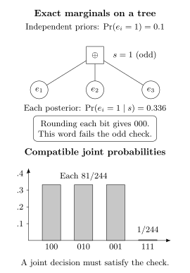
The check requires odd parity. Each bit individually is more likely to be zero, yet the all-zero word has posterior probability zero. The three single-error words are tied joint maxima. Correct local marginals are useful information, but they are not themselves a syndrome-consistent recovery.
BP with ordered-statistics decoding uses reliabilities to rank variables, solves an independent set of syndrome constraints, and searches selected changes to candidate assignments. It can repair an inconsistent BP output, though it does not generally compute the exact logical-class posterior. Roffe and collaborators (2020) study this approach across qLDPC examples. Iteration count, damping, search order and early stopping all affect its accuracy and runtime.
Tensor-network methods instead express class probabilities as sums over local fault variables. Approximate contraction controls the computational cost through parameters such as bond dimension. Renormalization methods combine local regions while passing effective probabilities between scales. They can retain degeneracy and correlations beyond a single-path approximation; finite approximation settings still need convergence checks. Chubb and Flammia (2021) develop statistical-mechanical formulations for correlated Pauli noise.
Learned decoders fit a map from measurement histories to decisions or class probabilities. They can use analog data and leakage indicators, as demonstrated by Bausch and collaborators (2024), but a numerical output between zero and one is not automatically a calibrated posterior. Calibration means that outcomes assigned a probability near occur with frequency near on suitable held-out data. Training and evaluation should be separated by independent runs when nearby shots share drift or hidden states.
Correlations and model mismatch
Section titled “Correlations and model mismatch”For CSS Codes, separate - and -component decoding is convenient. A physical error has both components, however, so their prior need not factorize. Joint Pauli messages, correlated matching or other joint methods can use information that independent decoders discard. Noise bias changes the appropriate weights, and persistent leakage can couple several successive rounds.
Detector means and pair correlations are helpful calibration statistics, but they do not determine a general joint distribution. For example, uniform distributions on the even-parity and odd-parity three-bit strings have the same individual means and pair correlations, yet opposite total parities. A model fitted only to pair statistics can miss precisely the higher-order feature relevant to a logical outcome.
The class-probability formulas also assume a stochastic fault model. Under coherent noise, amplitudes associated with the same measurement branch may interfere. Syndrome extraction does not automatically turn every coherent process into independent Pauli samples. Pauli Noise and Depolarizing Channels explains when a Pauli model is justified and what a twirling approximation discards.
Real-time decoding
Section titled “Real-time decoding”Throughput is the rate at which completed work can be sustained. Latency is the time from a record becoming available to its usable decision. A pipeline can have high throughput and long latency simultaneously.
If bits arrive every cycle of duration , the raw input rate is . For a standard stationary single-server queue with arrival rate and mean service time , stable stochastic operation requires load under the usual queueing assumptions. This mean-load test alone gives no deadline guarantee. Acquisition, transport, boundary reconciliation and actuation also contribute to the delay.
A useful requirement is a bound on the probability of missing the actual adaptive deadline:
For example, a stream arriving every microsecond can have mean service time microseconds yet occasionally require microseconds for one item. Its queue need not grow indefinitely, but a two-microsecond decision deadline can still fail.
Streaming decoders process new records incrementally. Windowed methods decode overlapping spacetime regions and delay decisions near uncertain boundaries. The overlap and commitment rule affect logical accuracy as well as latency. Receiving a final measurement can resolve an ambiguity that a shorter window could not.
Most inferred Pauli corrections can be tracked as a Pauli frame rather than physically applied. Clifford operations propagate that frame classically. This permits delayed decisions until an operation actually depends on them—for example, an adaptive non-Clifford measurement basis. Some surgery outcomes can likewise be tracked until their first dependent operation. There is no universal requirement to physically correct every cycle, nor unlimited freedom to postpone all inference.
To compare decoders, give them the same circuit, noise conditions and available measurements, then compare logical failure and timing on those same inputs. Count rejected runs and missing decisions as defined outcomes. A decoder with simulator-only fault labels is a reference bound, and an offline decoder can be an accuracy baseline without satisfying online deadlines. Logical Benchmarking develops uncertainty, acceptance and scaling comparisons.
Exercises
Section titled “Exercises”1. Recover the equivalence criterion
Section titled “1. Recover the equivalence criterion”If two Paulis have the same syndrome, why is in the normalizer? When are they equivalent recoveries?
Solution
For each stabilizer generator, commuting through the product gives two identical signs, whose product is positive. The product therefore commutes with every check and belongs to the normalizer. If it is a stabilizer up to phase, it acts trivially on the encoded state. A nontrivial logical Pauli in the normalizer instead changes the encoded information despite preserving the syndrome.
2. Choose the heavier repetition-code explanation
Section titled “2. Choose the heavier repetition-code explanation”For syndrome , take and . Which recovery is preferred, and what is its conditional success probability?
Solution
The probabilities are and . Correcting therefore succeeds conditionally with probability . The weight-one correction succeeds only with probability under this prior. Both candidates satisfy the observed checks.
3. Normalize the degenerate class probabilities
Section titled “3. Normalize the degenerate class probabilities”Use the two-qubit channel above to compare the overall success probability of the single-error MAP decoder and the logical-class decoder, including the even syndrome.
Solution
Identity is the only supported even-syndrome event, with probability . On the odd syndrome, single-error MAP chooses class A and succeeds on total probability ; class decoding chooses B and succeeds on total probability . Their overall successes are therefore and . Choosing class B need not identify whether or happened, since their actions differ only by a stabilizer and overall phase.
4. Interpret a negative edge weight
Section titled “4. Interpret a negative edge weight”An independent graph fault has , detector column and logical column . Replace its binary variable by . What changes besides the probability?
Solution
Now , so its weight is instead of . Over binary arithmetic , giving and . The observed detector pattern and reference logical label must therefore be offset by and . Taking the absolute weight without these offsets solves a different inference problem.
5. Calculate the exact one-check marginals
Section titled “5. Calculate the exact one-check marginals”For three independent bits of error probability conditioned on odd parity, derive the marginal . Check the result with one BP update.
Solution
Odd parity has probability . Bit 1 is one in the compatible words and , with combined probability . Their ratio is .
The prior LLR is , with . The odd check sends , so the posterior LLR is
Then . By symmetry every bit has this marginal. Rounding them independently gives the forbidden word ; the exact marginals were not the mistake.
6. Find a deadline failure in a stable stream
Section titled “6. Find a deadline failure in a stable stream”Items arrive at times microseconds. In every ten-item block, the first service takes microseconds and each other service takes . A first-in-first-out server starts empty. Find the mean service time and the first four latencies. Does a two-microsecond deadline always pass?
Solution
The mean service time is microseconds. The first completion times are , giving latencies . The queue subsequently clears before the next long item. Throughput is adequate, but one item in each block misses the two-microsecond deadline. A mean-speed statement would hide that failure.
7. Quantify a lost Pauli correlation
Section titled “7. Quantify a lost Pauli correlation”Let . Compare the true probability of simultaneous binary components with a product-of-marginals model.
Solution
The two component probabilities are and . Their product is , whereas the true joint probability is , thirty times larger. The covariance is . Treating the components independently changes the relative likelihoods of fault histories, even though it preserves both marginal error rates.
8. Show that pair statistics miss a logical feature
Section titled “8. Show that pair statistics miss a logical feature”Compare the uniform distributions on and . Calculate each bit mean, each distinct-pair product mean, and total parity.
Solution
In either distribution every bit is one in two of the four strings, so its mean is . Every distinct pair is jointly one in exactly one string, so its product mean is and its covariance is zero. Yet total parity is always even in the first distribution and always odd in the second. A decoder whose logical label depends on this parity needs information that pair statistics alone do not supply.
References
Section titled “References”- J. Bausch et al., “Learning high-accuracy error decoding for quantum processors,” Nature 635, 834–840 (2024), doi:10.1038/s41586-024-08148-8.
- S. Bravyi, M. Suchara, and A. Vargo, “Efficient algorithms for maximum likelihood decoding in the surface code,” Physical Review A 90, 032326 (2014), doi:10.1103/PhysRevA.90.032326, arXiv:1405.4883.
- C. T. Chubb and S. T. Flammia, “Statistical mechanical models for quantum codes with correlated noise,” Annales de l’Institut Henri Poincaré D 8, 269–321 (2021), doi:10.4171/AIHPD/105, arXiv:1809.10704.
- N. Delfosse and N. H. Nickerson, “Almost-linear time decoding algorithm for topological codes,” Quantum 5, 595 (2021), doi:10.22331/q-2021-12-02-595.
- O. Higgott and C. Gidney, “Sparse blossom: correcting a million errors per core second with minimum-weight matching,” Quantum 9, 1600 (2025), doi:10.22331/q-2025-01-20-1600, arXiv:2303.15933.
- D. Poulin and Y. Chung, “On the iterative decoding of sparse quantum codes,” Quantum Information and Computation 8, 987–1000 (2008), doi:10.26421/QIC8.10-8, arXiv:0801.1241.
- J. Roffe, D. R. White, S. Burton, and E. Campbell, “Decoding across the quantum low-density parity-check code landscape,” Physical Review Research 2, 043423 (2020), doi:10.1103/PhysRevResearch.2.043423, arXiv:2005.07016.