Quantum LDPC Codes

A quantum low-density parity-check code, or qLDPC code, has a sparse description: each chosen stabilizer check touches few qubits, and each qubit belongs to few checks. Sparsity can reduce the work needed to measure a syndrome and update a decoder. It does not by itself guarantee high encoding rate, large distance, short-range hardware connections, or a correct measurement schedule.

The most useful way to learn the subject is to separate three questions. What quantum code do the sparse matrices define? How do its parameters scale as the block grows? How can its checks and logical operations be implemented with noisy devices? We begin with a small matrix example, then construct hypergraph-product codes and examine the additional circuit constraints.

Required background. Why QEC Is Possible explains how checks preserve logical information. Stabilizer Formalism supplies commutation and distance, while Common Noise Models distinguishes independent errors from correlated faults.

Helpful background. CSS Codes explains the binary matrices used below.

Sparse Checks and Tanner Graphs

For a family of stabilizer codes, let $w_n$ be the maximum weight of a chosen generator and $\Delta_n$ the maximum number of those generators containing one qubit. The qLDPC requirement is

$$\sup_n w_n<\infty, \qquad \sup_n\Delta_n<\infty.$$

Both bounds must be independent of block length $n$. A finite matrix alone does not establish an asymptotic family. The requirement is that a sparse generating presentation exists; multiplying generators together can make a dense presentation of the same code.

For CSS codes, rows of $H_X$ and $H_Z$ specify positive $X$ and $Z$ checks. Their orthogonality condition and dimension are

$$\begin{aligned} H_XH_Z^{\mathsf T}&=0\pmod2,\\ k&=n-\operatorname{rank}H_X -\operatorname{rank}H_Z. \end{aligned}$$

Commutation requires even overlap between every opposite-type pair. The ranks count independent constraints; the number of measured rows can be larger. When defining $\Delta_n$, count incidences from both Pauli sectors.

A Tanner graph draws one node for each check and one for each qubit, joining them whenever the matrix entry is one. Check weight is a check-node degree. Qubit participation is a qubit-node degree. For example, use the same matrix in both sectors:

$$\begin{aligned} H_X&=H_Z=M,\\ M&= \begin{pmatrix} 1&1&1&1&0&0&0&0\\ 0&0&1&1&1&1&0&0\\ 0&0&0&0&1&1&1&1 \end{pmatrix}. \end{aligned}$$

Every row has weight four, distinct rows overlap on zero or two positions, and $MM^{\mathsf T}=0$. The rank is three, so this block encodes $8-3-3=2$ qubits. The largest total qubit degree is four: a middle qubit participates in two $X$ and two $Z$ checks.

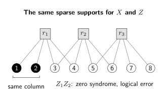
One Tanner graph for the matrix $M$; the same supports are used in both Pauli sectors. Squares are checks, circles are qubits. Qubits 1 and 2 have identical columns, so a $Z_1Z_2$ error has zero $X$-check syndrome. Here it is a nontrivial logical operator: the sparse block has distance two. A sparse drawing alone is not a distance guarantee.

The first two columns coincide, so $Z_1Z_2$ commutes with all checks. Its support is not in the row space of $M$, making it a nontrivial logical operator. No single-qubit Pauli commutes with every check because every column is nonzero in both sectors. Hence the block has parameters $[[8,2,2]]$. Repeating disjoint copies would produce a constant-rate qLDPC family with distance still two, illustrating why sparsity and protection must be tested separately.

Sparsity nevertheless has concrete benefits. There are $O(n)$ check–qubit edges, so a local message-passing iteration can take $O(n)$ work. A weight-$w$ check needs only $w$ data–ancilla interactions in a basic extraction circuit. Neither statement bounds the number of decoding iterations, routing time, or correlated errors produced by a faulty ancilla.

Rate and Distance as the Block Grows

For parameters $[[n,k,d]]$, the rate is $R_n=k/n$ and the relative distance is $\delta_n=d/n$. A family is asymptotically good when both remain bounded away from zero, equivalently $k=\Theta(n)$ and $d=\Theta(n)$. This is stronger than constant rate alone.

Family parameters	Rate	Relative distance
$[[2L^2,2,L]]$	$1/L^2$	$1/(2L)$
$[[n,n/5,\sqrt n]]$	$1/5$	$1/\sqrt n$
$[[n,n/5,n/20]]$	$1/5$	$1/20$

Assume compatible block lengths and bounded check degrees in the last two schematic examples. The first is the toric family; the second has constant rate but vanishing relative distance; the third is asymptotically good. The existence of asymptotically good qLDPC families is an established theorem, proved by Panteleev and Kalachev using lifted products. It is not a claim that every finite block in those constructions has favorable practical constants.

The quantum Singleton bound gives $n-k\ge2(d-1)$. Thus, when rate and relative distance have limits, $R+2\delta\le1$. Increasing one limits the other even before sparse-check or hardware constraints are imposed.

The two-dimensional locality tradeoff, $kd^2\le Cn$, is stronger but has additional assumptions: bounded local dimension, spatial density, and interaction range in a Euclidean plane, with commuting-projector constraints. It is not a bound on every sparse graph. High-rate codes with growing distance must use connectivity or other structure outside those assumptions. A few distant qubits still form a low-weight check; their geometric separation remains a physical cost.

Building a Hypergraph-Product Code

Tillich and Zémor’s hypergraph product builds commuting quantum checks from two classical binary matrices, without requiring the seeds to be mutually orthogonal. Let $H_i$ have $r_i$ rows and $n_i$ columns. There are two groups of quantum coordinates, of sizes $n_1n_2$ and $r_1r_2$.

Define the two blocks of each check matrix by

$$\begin{aligned} A_X&=H_1\otimes I_{n_2},\\ B_X&=I_{r_1}\otimes H_2^{\mathsf T},\\ A_Z&=I_{n_1}\otimes H_2,\\ B_Z&=H_1^{\mathsf T}\otimes I_{r_2}. \end{aligned}$$

Then $H_X=[A_X\mid B_X]$ and $H_Z=[A_Z\mid B_Z]$. The tensor product replicates each seed incidence while keeping track of the coordinate in the other seed. The two contributions to the commutator agree and cancel over $\mathbb F_2$:

$$H_XH_Z^{\mathsf T} =H_1\otimes H_2^{\mathsf T} +H_1\otimes H_2^{\mathsf T}=0.$$

Write $k_i=\dim\ker H_i$ and $k_i^T=\dim\ker H_i^{\mathsf T}$. The latter counts independent relations among seed rows. The resulting quantum parameters satisfy

$$\begin{aligned} n&=n_1n_2+r_1r_2,\\ k&=k_1k_2+k_1^Tk_2^T. \end{aligned}$$

The transpose term matters when both seeds have redundant rows. This is one reason replacing a seed by an equivalent classical parity-check matrix need not leave its quantum product unchanged: the product uses the matrix and its transpose, not only the classical kernel.

Let $d_i$ and $d_i^T$ be the minimum nonzero weights in the two seed kernels, setting the distance to infinity for a zero-dimensional kernel. The general product bound is

$$d\ge\min(d_1,d_2,d_1^T,d_2^T).$$

With full-row-rank seeds that both encode nonzero classical dimensions, the transpose kernels vanish and equality gives $d=\min(d_1,d_2)$. Suitable bounded-degree seeds with constant classical rate and distance proportional to their length yield quantum constant rate and distance proportional to $\sqrt n$.

A product small enough to verify

Choose identical repetition seeds

$$H_1=H_2=\begin{pmatrix}1&1&0\\0&1&1\end{pmatrix}.$$

Their kernels are $\{000,111\}$, their ranks are two, and their transpose kernels are trivial. Hence the product gives

$$[[n,k,d]]=[[13,1,3]].$$

An $X$-check row has weight two from $H_1$ plus one or two from a column of $H_2$, so its weight is three or four. The same holds in the other sector. Each quantum coordinate participates in at most four checks total. The resulting 12 rows are independent; their rank is 12, not an assumed consequence of merely counting them.

For a geometric family, instead use the cyclic repetition matrix $I+P_L$, where $P_L$ shifts a length-$L$ bit string by one position and $L\ge3$. Its kernel and transpose kernel each have dimension one and distance $L$. The product gives $[[2L^2,2,L]]$, recovering the toric family. The extra transpose contribution is exactly the second logical qubit.

Other Constructions and What Their Theorems Say

The hypergraph product is a useful starting point, not a ceiling on qLDPC distance. Quantum expander codes use suitable seed expansion to obtain provable decoding guarantees. Lifted-product and quantum Tanner constructions achieve constant rate and linear distance under their respective algebraic and local-code conditions. The proofs concern whole families and specified decoders; their constants and required block sizes still matter in applications.

Quasi-cyclic constructions give compact finite matrices using sparse shift operators. For commuting square binary matrices $A,B$, the form

$$\begin{aligned} H_X&=[A\mid B],\\ H_Z&=[B^{\mathsf T}\mid A^{\mathsf T}] \end{aligned}$$

commutes because $H_XH_Z^{\mathsf T}=AB+BA=0$. Bivariate-bicycle codes take structured polynomials in two commuting cyclic shifts. Choosing a fixed number of shift terms bounds row and column weights, but does not alone prove distance.

Bravyi and collaborators’ circuit-level study includes a $[[144,12,12]]$ block with weight-six checks and a proposed circuit using 144 data qubits plus 144 measurement ancillas. The code’s data rate is $1/12$; including those ancillas gives 24 physical qubits per encoded qubit. These counts describe that design. They do not include every routing, control, or logical-operation cost and are not themselves an experimental threshold. Dated hardware and scaling comparisons are discussed in Quantum LDPC and High-Rate Codes.

Decoding and Noisy Check Outcomes

For a $Z$-error vector $e_Z$, the perfect $X$-check syndrome is $s_X=H_Xe_Z^{\mathsf T}$. Successful recovery needs $r_Z+e_Z$ in the row space of $H_Z$, not necessarily $r_Z=e_Z$. Stabilizers make different microscopic errors equivalent on encoded states. The analogous statement holds for $X$ errors.

The maximum-likelihood objective therefore sums probabilities within each compatible logical class. A class containing the most likely individual error need not have the largest total probability. Conversely, two large probabilities in one class cannot settle the comparison if the other class’s remaining probability is unknown. Exercise 6 makes that missing-information issue explicit.

Belief propagation passes local probability messages on a Tanner graph. On a tree, the usual messages can yield exact marginals. Quantum check commutation introduces overlapping supports; in the combined $X/Z$ graph, a shared pair of qubits gives a four-cycle. Individual-sector graphs may have different cycles. Messages on loopy graphs are correlated and can stall or produce a syndrome-inconsistent estimate. Quantum degeneracy creates an additional challenge beyond ordinary classical decoding.

Roffe and collaborators study belief propagation with ordered-statistics post-processing: reliability estimates guide a subsequent syndrome-solving search. This can repair a failed message-passing result, at additional computational cost. Linear work per iteration does not imply linear total runtime if iteration counts or post-processing grow. For a real-time memory, runtime tails and missed deadlines matter alongside logical failure probability.

With measurement errors, a simplified report is $\widetilde s=He^{\mathsf T}+\eta$, where $\eta$ is readout noise. If a binary row-relation matrix $D$ satisfies $DH=0$, then

$$D\widetilde s=D\eta.$$

The relation can reveal an inconsistent report, but need not identify the bad bit. One parity relation detects an odd number of flipped reports and misses even patterns. More redundancy is not automatically single-shot correction. In a single-shot scheme, a bounded number of noisy measurement rounds leads to controlled residual data noise under the stated model, so correction can be repeated reliably as the code grows. That stronger property needs a specific construction and decoder; Bombín’s single-shot work is one such mechanism.

A Sparse Schedule Must Measure the Right Observables

Attach a distinct ancilla to every simultaneously measured check. The check–data incidence graph is bipartite. If its maximum degree is $D_{\max}=\max(w,\Delta)$, bipartite edge coloring partitions its interactions into $D_{\max}$ layers with no shared-qubit collision. This is a statement about available gate slots, not yet about the implemented measurement.

The distinction appears even with two data qubits. To measure $X_1X_2$, prepare ancilla $a$ in $|+\rangle$, apply CNOTs $a\to1$ and $a\to2$, and measure $X_a$. To measure $Z_1Z_2$, prepare $b$ in $|0\rangle$, apply $1\to b$ and $2\to b$, and measure $Z_b$. The two observables commute. But their component CNOTs can fail to commute when interleaved.

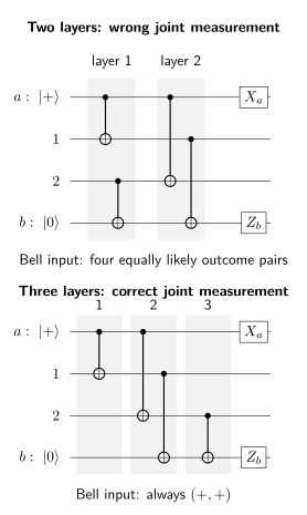
Both schedules contain the same four CNOTs and avoid shared-qubit gate collisions. The upper order does not jointly measure $X_1X_2$ and $Z_1Z_2$ as intended. For data in $|\Phi^+\rangle$, it entangles the two ancillas and produces all four outcome pairs equally often. The lower order gives the correct deterministic $(+,+)$ outcomes. Preparation and readout are fixed as labeled; the comparison concerns ideal gate ordering before any noise is added.

The incorrect order places $a\to1$ before $1\to b$, but $2\to b$ before $a\to2$. The contributions through the shared data qubits no longer cancel, leaving an unwanted ancilla coupling. The three-layer order keeps the $X$-ancilla interaction before the $Z$-ancilla interaction on both shared data qubits. Exercise 5 verifies the output states directly.

For one Pauli sector, the basic CNOTs commute, so edge coloring does give a valid ideal interaction schedule. Measuring all $X$ checks and then all $Z$ checks supplies a simple constant-layer baseline when both degree bounds are fixed and every required edge is available. More efficient interleaving must preserve the complete measurement instrument. Fault-tolerant scheduling imposes further conditions on ancilla-error propagation, verification or flags, and repeated-round detectors. The explicit bivariate-bicycle schedules in Bravyi and collaborators’ study illustrate this extra circuit design.

Routing, shuttling, long-range couplers, preparation, reset, leakage handling, and limited parallel control can add time beyond this ideal graph calculation. Code distance counts data-Pauli support; circuit distance counts the smallest allowed fault set causing an undetected logical effect in the chosen circuit and temporal boundaries. Bounded check weight does not make those distances equal.

Comparing Encoded Blocks

A high-rate block stores several logical qubits whose errors may be correlated. In a stochastic logical-Pauli model, let $P_{\rm block}$ be the probability of any nonidentity logical action and $p_j$ the marginal probability of a nonidentity action on logical qubit $j$. Then

$$\max_j p_j\le P_{\rm block}\le\sum_j p_j.$$

Dividing block failure by $k$ does not generally recover a marginal error probability. Independent rare failures and simultaneous block-wide failures can have identical marginals but very different block probabilities. Coherent logical channels additionally require channel-based metrics rather than an assumed classical failure distribution.

Resource comparisons should include the full extraction and logical-operation procedure. Data rate can improve while ancilla count, cycle time, communication, or decoding cost increases. Many-qubit blocks also need a way to initialize, address, entangle, and measure selected logical qubits; a memory simulation alone does not supply a universal gate set. Resource Estimation explains how to compare those costs for a specified computation.

Distance values also have different strengths. A found nontrivial logical operator proves an upper bound on distance. A lower-bound theorem excludes all smaller logicals. An exhaustive search or matching upper and lower bounds can establish the exact distance. A fitted logical-error exponent under one decoder is not a substitute for these algebraic statements.

Exercises

1. Sparse does not imply growing distance

Find $w,\Delta,k,d$ for the eight-qubit matrix $M$, then repeat independent copies. What happens to rate and distance?

Solution

The rows have weight four, and middle columns have weight two in each sector, so $w=4$ and total $\Delta=4$. The three rows are independent, giving $k=2$. Every column is nonzero, excluding weight-one logical Paulis. The vector $11000000$ has zero syndrome but is not in the row space, so $Z_1Z_2$ is a logical operator and $d=2$. With $b$ copies, parameters are $[[8b,2b,2]]$. The rate stays $1/4$ while relative distance tends to zero.

2. Count a product without assuming distance

Let $H_1$ be $6\times10$ of rank six and $H_2$ be $4\times7$ of rank four. Find $n,k$. What can be concluded about distance from these facts alone?

Solution

The product length is $10(7)+6(4)=94$. Seed kernel dimensions are four and three, and both transpose kernels vanish, giving $k=4(3)=12$. The exact distance is the smaller of the two seed distances in this full-row-rank, nonzero-kernel case. Shapes and ranks alone do not determine those distances. Full row rank does not exclude a zero column and a weight-one seed codeword.

3. Redundant seed checks change the product

Compare identical length-three repetition seeds chosen as the $2\times3$ open-chain matrix above or the $3\times3$ cyclic matrix $I+P_3$. Both define the classical kernel $\{000,111\}$. Find their quantum product parameters.

Solution

The open-chain seed has rank two, kernel dimension one, and transpose-kernel dimension zero. Its product has $n=9+4=13$, $k=1$, and $d=3$. The cyclic seed also has rank two and the same kernel, but its three rows have one relation. Both kernel dimensions are now one, giving $n=9+9=18$, $k=1+1=2$, and $d=3$. The product construction depends on the full seed complex, including relations among rows.

4. What one syndrome relation can reveal

Three measured binary checks satisfy $s_1+s_2+s_3=0$. For reported bits $\widetilde s=s+\eta$, what is learned from their parity? Can it locate one wrong report?

Solution

The observed parity is $\eta_1+\eta_2+\eta_3$. A single wrong report gives one, so it is detected, but all three possible locations give the same result. Two wrong reports give zero and evade this test. The single relation alone therefore neither corrects arbitrary readout errors nor establishes single-shot quantum correction.

5. Test the two gate orders

Use data $|\Phi^+\rangle=(|00\rangle+|11\rangle)/\sqrt2$ and ancillas $a=|+\rangle,b=|0\rangle$. Calculate the final state before ancilla readout for each schedule in the figure.

Solution

Write the initial computational values as $a=u$, $1=2=t$, $b=0$, with a uniform coherent sum over $u,t\in\{0,1\}$. The two-layer schedule gives $1=2=t+u$ and $b=u$, with addition modulo two. Changing variable to $t+u$ shows that the final state factors as

$$|\Phi^+\rangle_{12}\otimes|\Phi^+\rangle_{ab}.$$

Measuring $X_a$ and $Z_b$ on this ancilla Bell pair gives each sign pair with probability $1/4$, although both data checks equal $+1$. In the lower schedule, both data interactions with $a$ precede their interactions with $b$. Thus $b=(t+u)+(t+u)=0$, and the state is

$$|\Phi^+\rangle_{12}\otimes|+\rangle_a|0\rangle_b.$$

The outcomes are deterministically $(+,+)$. Avoiding simultaneous gate collisions was necessary but insufficient.

6. Incomplete probabilities do not rank logical classes

Two stabilizer-equivalent errors in class $A$ have conditional probabilities $0.15$ and $0.12$. One error in another class $B$ has probability $0.20$. Can these facts alone determine which class is more likely? Give two complete distributions with opposite answers.

Solution

Only lower bounds are known: $P(A\mid s)\ge0.27$ and $P(B\mid s)\ge0.20$. There is $0.53$ unassigned probability. Assign it to four additional distinct errors of probability $0.1325$ each in $A$; then the class totals are $(0.80,0.20)$. Assign those four errors instead to $B$; the totals become $(0.27,0.73)$. Other compatible errors can have zero probability in these toy distributions, and the classes are assumed large enough to contain the listed errors. In both cases the $0.20$ error remains the largest individual term, but its class wins only in the second distribution.

7. Marginal and block failure

In a stochastic logical model, each of 12 logical qubits has marginal failure probability $p=0.001$. Compare independent failures with perfectly correlated failures of all 12 together.

Solution

Independence gives $P_{\rm block}=1-(1-p)^{12}\approx0.01193$. A single common event flipping all 12 gives $P_{\rm block}=p=0.001$. Both have the same marginal $p$, and both satisfy $p\le P_{\rm block}\le12p$. Dividing the correlated block probability by 12 would understate every marginal by a factor of 12. The joint logical distribution matters.

References

• H. Bombín, “Single-shot fault-tolerant quantum error correction,” Physical Review X 5, 031043 (2015), doi:10.1103/PhysRevX.5.031043, arXiv:1404.5504.
• S. Bravyi et al., “High-threshold and low-overhead fault-tolerant quantum memory,” Nature 627, 778–782 (2024), doi:10.1038/s41586-024-07107-7, arXiv:2308.07915.
• A. Leverrier, J.-P. Tillich, and G. Zémor, “Quantum expander codes,” in 2015 IEEE 56th Annual Symposium on Foundations of Computer Science, 810–824 (2015), doi:10.1109/FOCS.2015.55, arXiv:1504.00822.
• A. Leverrier and G. Zémor, “Quantum Tanner codes,” in 2022 IEEE 63rd Annual Symposium on Foundations of Computer Science, 872–883 (2022), doi:10.1109/FOCS54457.2022.00117, arXiv:2202.13641.
• P. Panteleev and G. Kalachev, “Asymptotically good quantum and locally testable classical LDPC codes,” in Proceedings of STOC 2022, 375–388 (2022), doi:10.1145/3519935.3520017, arXiv:2111.03654.
• J. Roffe, D. R. White, S. Burton, and E. T. Campbell, “Decoding across the quantum low-density parity-check code landscape,” Physical Review Research 2, 043423 (2020), doi:10.1103/PhysRevResearch.2.043423, arXiv:2005.07016.
• J.-P. Tillich and G. Zémor, “Quantum LDPC codes with positive rate and minimum distance proportional to the square root of the blocklength,” IEEE Transactions on Information Theory 60, 1193–1202 (2014), doi:10.1109/TIT.2013.2292061, arXiv:0903.0566.

Further Reading

• N. P. Breuckmann and J. N. Eberhardt, “Quantum low-density parity-check codes,” PRX Quantum 2, 040101 (2021), doi:10.1103/PRXQuantum.2.040101 — an introduction to sparse-code constructions; its historical survey predates the asymptotically good constructions cited above.