Quantum LDPC and High-Rate Codes

High-rate quantum codes can protect many logical qubits in one block. Their attraction is lower storage cost, but an algorithm also needs noisy check measurements, timely decoding and operations on selected logical qubits. This page follows a finite block from its code parameters to those physical requirements.

The qLDPC research assessment discusses selected constructions and experiments with a retained historical cutoff of 11 August 2026. The examples here explain stable comparisons; their added hardware counts and timings are illustrative assumptions.

Helpful background. Quantum LDPC codes defines sparse checks, rate, distance and logical-class decoding. Stabilizer formalism supplies the algebra; surface codes provides a local reference; resource estimation connects protected operations to a workload.

High rate is a statement about a code family

A quantum LDPC family has check weights and the number of checks touching each qubit bounded independently of block length $n$. A constant-rate family additionally has $k=\Theta(n)$ encoded qubits. An asymptotically good family also has distance $d=\Theta(n)$.

Panteleev and Kalachev proved that asymptotically good qLDPC families exist; Leverrier and Zémor gave a quantum Tanner-code construction with the same qualitative rate–distance scaling. Panteleev and Kalachev (2022), Leverrier and Zémor (2022) This settles a code-existence question. It does not specify a small practical constant, an extraction circuit, or a complete universal computer.

The distinction matters even before hardware is considered. A constant-rate family can have poor or even constant distance. A single impressive $[[n,k,d]]$ block does not establish a family with good scaling. Finally, the data ratio $n/k$ says nothing by itself about the number of ancillas, routing systems or logical operations needed at the requested error rate.

Whole blocks create a finite-size cost

If each block encodes $k$ logical qubits and a task needs $Q$ simultaneously, its data count is

$$N_{\rm data}=n\left\lceil\frac Qk\right\rceil.$$

The ceiling matters when blocks are only partly occupied. The ratio approaches $n/k$ when many blocks are filled, but not when most encoded capacity is unused.

Take a $[[144,12,12]]$ block. A published bivariate-bicycle memory construction uses 144 data and 144 check qubits for this code. Bravyi et al. (2024) For this illustrative calculation, add 24 routing or buffer qubits per block. The counted footprint becomes

$$N_{\rm counted}=312\left\lceil\frac Q{12}\right\rceil.$$

Twelve logical qubits fit in one block, costing 312 physical qubits in this model. Thirteen require two blocks and cost 624. Using all 24 logical positions returns the ratio to 26 physical qubits per served logical qubit. Spare capacity and factories have not yet been included.

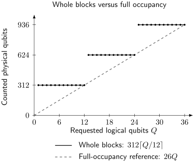
Finite-block occupancy in the illustrative model: each block serves at most 12 logical qubits and costs 312 physical qubits. Dots show integer requested widths. The dashed line, $26Q$, is the fully occupied reference, not an available fractional-block implementation. Unused logical positions explain the gap; factories and spares would add further cost.

A fair comparison uses enough local-code patches to serve the same $Q$, at the same reliability and elapsed time. It also counts corresponding ancillary resources on both sides. Comparing one multi-logical block with one single-logical patch answers a different question.

Block failure is not marginal failure

Let $L_j$ be failure of logical qubit $j$ in a specified task. With marginal probabilities $p_j$, the probability that at least one fails satisfies

$$\max_jp_j\leq P_{\rm block} \leq\min\left(1,\sum_jp_j\right).$$

These bounds need no independence. If all $k$ failures are independent with probability $p$, then $P_{\rm block}=1-(1-p)^k$. The approximation $kp$ requires small $kp$; weakly described “correlations” are not a substitute for a model.

Consider two logical qubits, each failing with probability $p=0.01$. Independent failures give $P_{\rm block}=0.0199$ and probability $0.0001$ that both fail. A shared event that always damages both gives $P_{\rm block}=0.01$, but probability $0.01$ that both fail. The correlated channel has fewer failing blocks and more simultaneous damage. Neither one number nor the average marginal rate describes every workload.

For that reason, a multi-logical code comparison should identify the logical error patterns that affect the computation. A decoder returning a correction with the measured syndrome may still leave a nontrivial logical operator. The code foundations explain how to test the residual modulo stabilizers.

Compare storage at the same elapsed time

A syndrome cycle is a procedure, not a universal unit of time. Its duration includes required preparation, interactions, movement, measurement and any feedback that cannot be deferred. Overlapping or pipelined stages follow their dependency schedule; not every decoder latency must be added to every cycle.

For a simple model where a block survives each cycle independently with probability $1-p$, the probability of at least one failure in $m$ cycles is

$$P_{\rm fail}(m)=1-(1-p)^m.$$

This treats failure as an absorbing event. If later logical flips can cancel before final measurement, endpoint error follows a different law. At elapsed time $t=m\tau$, the absorbing model has rate

$$\gamma=-\frac{\ln(1-p)}{\tau},$$

approximately $p/\tau$ at small $p$. A longer cycle with the same per-cycle failure has a lower rate by this definition. In real hardware, increasing cycle duration can increase $p$ through additional idling and control errors; those changes must be modeled, not inferred from duration alone.

Likewise, qubit-time per cycle is not qubit-time for a matched memory task. A 288-qubit design taking ten microseconds per cycle and a 3000-qubit design taking one microsecond have similar qubit-time per cycle. Over the same one-millisecond storage interval, their occupied qubit-times differ by a factor of $3000/288\approx10.42$. Whether either meets the required reliability is a separate calculation.

Which decoders can scale?

Sparse checks limit the work of one message-passing iteration, not necessarily the number of iterations or the cost of a difficult syndrome. Belief propagation with ordered-statistics post-processing is a useful finite-code approach: soft information guides a search for a syndrome-consistent correction. Its accuracy and cost depend on the code, noise model, iteration limits and search order. Roffe et al. (2020)

Four quantities answer different questions: logical error, sustained throughput, latency distribution and memory use. A fast median can coexist with long delays on rare syndromes. A low logical error obtained without a time limit may be unsuitable when an adaptive operation has a deadline. Conversely, a delayed Pauli-frame update can be acceptable if no pending operation needs it yet.

For $B$ blocks emitting $m$ records each every cycle of duration $\tau$, the input rate is $Bm/\tau$. With bounded nontrivial check weight and bounded qubit participation, the chosen syndrome representation has $O(n)$ incidences and at most $O(n)$ checks per block. This controls one input-size scaling; it does not prove linear-time decoding.

Localization, parallelism and learned models can reduce practical cost. Their benefit must survive large connected fault clusters, missing checks and changes in the device noise. Proofs for a particular expander family and empirical performance on a different finite circuit answer different questions. See decoders and real-time control for the algorithms and timing requirements.

Can hardware realize the connectivity?

Bounded degree does not imply short edges. For geometrically local commuting constraints on a two-dimensional lattice with bounded local dimension and range, the tradeoff $kd^2=O(n)$ limits simultaneous rate and distance. Bravyi, Poulin and Terhal (2010) A constant-rate family with growing distance must leave some of those assumptions. Sparse nonlocal interactions are one route.

Thin planar connectivity constructions show how check graphs can be organized into a small number of planar layers. Tremblay et al. (2022) This is not the same as placing all qubits in one plane with every interaction of bounded geometric length.

How an interaction is supplied	What it can simplify	What remains physical
Fixed long-range couplers	Direct access to sparse distant neighbors	Coupler length, frequency crowding and simultaneous-gate errors
Motion or shared modes	Access without a fixed nearest-neighbor graph	Transport time, heating, spectators and limited parallelism
Heralded links between modules	Connections between separate processors	Random waiting time, stored-state decay and failed connections

A drawn layout establishes geometry under its design rules. It does not measure the resulting gate errors or device yield. Similarly, a collision-free gate schedule can still have incorrect ordering between overlapping $X$ and $Z$ check circuits; the qLDPC circuit example explains the additional commutation issue.

Compact storage still needs logical access

Several logical qubits share the same data block. Their logical Pauli representatives may overlap, so acting on a chosen coordinate is not automatically the same as acting on a separate patch. A code automorphism or transversal operation may transform many logical qubits together. An efficiently available global Clifford transformation need not allow every desired one-qubit operation at equal cost.

Teleportation, generalized surgery and logical-Pauli measurements can provide access using extra qubits and rounds. The expanded check circuit must retain the intended protection. Universal computation also needs a non-Clifford mechanism. These costs belong in a compiled-workload comparison, beyond the memory ratio $n/k$.

The fault-tolerant architecture page connects logical failure allowances, resource-state supply and feedback. The historical qLDPC assessment links specific logical-operation results with their assumptions.

Exercises

1. Include ancillary systems and spares

Ten blocks in the illustrated model serve 120 logical qubits. Add spare capacity equal to 10% of the counted subtotal. Find the footprint and qubits per served logical qubit.

Solution

The subtotal is $10\times312=3120$. Adding 312 spares gives 3432 physical qubits, or $3432/120=28.6$ per served logical qubit. The abstract data ratio $144/12=12$ omits both the check ancillas and the added implementation resources. No factory cost was specified.

2. Compute independent block failure

A block holds 12 logical qubits with independent failure probability $10^{-6}$ each in the specified trial. What is the probability that at least one fails?

Solution

It is $1-(1-10^{-6})^{12}\approx1.1999934\times10^{-5}$. The first-order value is $1.2\times10^{-5}$. Without independence, equal marginals alone permit a block probability between $10^{-6}$ and $12\times10^{-6}$. The lower extreme can occur when every failure damages all twelve logical qubits together.

3. Estimate sustained record throughput

Five hundred blocks emit 144 records each every millisecond. Compare their rate with a service capacity of $8.0\times10^7$ records per second.

Solution

The arrival rate is $7.2\times10^7$ records per second. Capacity exceeds arrivals by about 11.1% of the arrival rate, or 10% of capacity. That passes an average capacity check, but does not bound queue lengths or decision latency during bursts.

4. Interpret a latency quantile

A decoder has median latency $0.2\,\mathrm{ms}$ and 99.9th percentile $0.8\,\mathrm{ms}$. A particular decision is needed within $0.5\,\mathrm{ms}$. Is that deadline established?

Solution

No. The two quoted quantiles do not determine the probability of exceeding $0.5\,\mathrm{ms}$. Measure that tail and specify the response to a late decision. A safe pause can turn a potential failure into extra runtime and memory exposure; if the protocol cannot pause, the deadline is a reliability requirement.

5. Normalize to elapsed storage time

Two hypothetical blocks each have absorbing failure probability $10^{-6}$ per cycle. Their cycles take ten microseconds and one microsecond. Find their failure probabilities over one millisecond under the independent-cycle model.

Solution

The slower block has 100 cycles and probability approximately $9.999505\times10^{-5}$. The faster one has 1000 cycles and probability approximately $9.995007\times10^{-4}$. In this deliberately fixed-per-cycle model, the faster cycle repeats the specified failure opportunity more often. A physical comparison must recalculate each per-cycle probability from its actual duration and noise; neither speed alone nor per-cycle error alone decides the result.

6. Keep acceptance separate from state quality

A four-millisecond preparation attempt accepts with probability 0.25. Among accepted states, a specified binary verification test fails with probability $10^{-5}$. Find the accepted-output rate and probability that an attempt both accepts and passes that test.

Solution

The accepted rate is $0.25/0.004=62.5$ per second. The joint accept-and-pass probability is $0.25(1-10^{-5})=0.2499975$. This is a statement about the named test; an arbitrary quantum-state infidelity cannot be silently substituted for a recognized binary failure probability.

7. Is a partial comparison an upper bound?

A local reference uses $8N$ data qubits. A candidate uses $N$ data qubits, $N$ check ancillas and $2N$ routing qubits, plus 25% spares on that subtotal. Is its maximum possible total saving a factor of 1.6?

Solution

The candidate’s stated count is $5N$, so $8N/(5N)=1.6$ compares the reference’s data only with the candidate’s stated total. It is not an upper bound on the complete ratio. Reference ancillas can raise the numerator, while omitted candidate factories can raise the denominator. For example, reference total $16N$ gives a factor 3.2 if $5N$ is the full candidate total. Complete both counts before comparing them.

8. Identify unused logical capacity

Using the figure’s model, compare serving 12 and 13 logical qubits. Could the spare encoded positions in the second case be useful?

Solution

The counts are 312 and 624, giving 26 and 48 physical qubits per requested logical qubit. The second block leaves eleven logical positions unused by this storage request. A workload might use them for other data or operations, but that requires a compatible schedule and logical access. They cannot be counted as both occupied service and free resources without specifying the assignment.

References

• S. Bravyi, A. W. Cross, J. M. Gambetta, D. Maslov, P. Rall, and T. J. Yoder, “High-threshold and low-overhead fault-tolerant quantum memory,” Nature 627, 778–782 (2024). doi:10.1038/s41586-024-07107-7.
• S. Bravyi, D. Poulin, and B. M. Terhal, “Tradeoffs for reliable quantum information storage in 2D systems,” Physical Review Letters 104, 050503 (2010). doi:10.1103/PhysRevLett.104.050503.
• A. Leverrier and G. Zémor, “Quantum Tanner codes,” in Proceedings of FOCS 2022, 872–883 (2022). doi:10.1109/FOCS54457.2022.00117.
• P. Panteleev and G. Kalachev, “Asymptotically good quantum and locally testable classical LDPC codes,” in Proceedings of STOC 2022, 375–388 (2022). doi:10.1145/3519935.3520017.
• J. Roffe, D. R. White, S. Burton, and E. T. Campbell, “Decoding across the quantum low-density parity-check code landscape,” Physical Review Research 2, 043423 (2020). doi:10.1103/PhysRevResearch.2.043423.
• M. A. Tremblay, N. Delfosse, and M. E. Beverland, “Constant-overhead quantum error correction with thin planar connectivity,” Physical Review Letters 129, 050504 (2022). doi:10.1103/PhysRevLett.129.050504.