Fault-Tolerant Quantum Computing Frontier

A fault-tolerant computer must preserve quantum information while transforming it. Its code, syndrome measurements, decoder, logical gates, resource-state preparation and control must work together throughout the intended calculation. A good logical memory is one essential component; it does not specify the performance of an entire algorithm.

This page develops those connections with simplified models. For selected experimental results, see the fault-tolerant computing assessment, which explicitly retains a historical cutoff of 11 August 2026.

Helpful background. Stabilizer formalism and the surface code explain encoded information and repeated checks. Fault-tolerant gates explains controlled error propagation. Resource estimation develops the detailed conversion from a logical schedule to hardware and runtime.

A memory, a logical gate and a computation test different things

A memory test asks whether an unknown encoded state survives a specified duration. A logical gate also changes the information, often through extra ancillas, joint measurements or adaptive operations. A long computation repeats many such steps and may expose faults too rare to resolve in a small demonstration.

Two useful comparisons must remain distinct. Break-even means outperforming a specified physical reference on a matched task. Error suppression with increasing protection means that larger distance or another protection parameter reduces logical failure over the tested range. A system can demonstrate one without establishing the other. Neither is a guarantee that an extrapolated error law continues indefinitely. Error-correction case studies shows how these comparisons are made.

Universality is another separate question. A fixed exact code on finitely many finite-dimensional subsystems, detecting arbitrary errors on each subsystem, cannot implement a universal gate set solely by transversal encoded unitaries. Eastin and Knill (2009) Architectures therefore add mechanisms such as magic-state-assisted operations or switching between codes. Transversal gates on different codes can contribute to a universal construction, but the switching operations also require fault protection.

Magic states together with appropriate Clifford operations provide one route to universality. Bravyi and Kitaev (2005) A useful machine must supply those states with adequate quality and timing; demonstrating improved state fidelity alone does not determine that supply.

A code changes where the hardware cost appears

A code specifies how information is encoded and which errors can be corrected. Hardware supplies interactions, measurements and reset. The mapping between them matters as much as the abstract code parameters.

Choice	Benefit and remaining cost
Two-dimensional surface-code patches	Local checks and well-developed logical operations; count patch size, routing space and resource-state factories.
High-rate quantum LDPC blocks	Many logical qubits in one protected block; count long-range interactions, syndrome circuits and access to individual logical qubits.
Bosonic encoding with an outer code	Suppress or reveal dominant oscillator faults before outer correction; count oscillator control, ancillary systems and residual error channels.
Networked modules	Connect smaller processors through shared entanglement; count probabilistic delivery, memory aging, buffering and communication faults.

Quantum LDPC means bounded check weight and bounded participation of each qubit as the code family grows. It does not mean that checks are geometrically local. The architectural obstacle can be the length and scheduling of interactions even when graph degree stays bounded. See high-rate codes.

For bosonic encodings, a mode is not interchangeable with a two-level qubit in a hardware count. For networked modules, the mean entanglement rate does not specify delivery by a deadline. Compare alternatives at the same logical task and accuracy, including their different physical resources. The layered framework of Beverland et al. (2022) makes these conversions explicit.

The workload sets the required logical reliability

Suppose a stochastic failure model identifies $N_j$ relevant opportunities of type $j$, each with probability at most $p_j$. If every failure of the requested calculation is covered by at least one of these events, the union bound gives

$$P_{\rm fail}\leq\sum_j N_jp_j.$$

The bound needs no independence. It is conservative because events can overlap and some counted faults may not spoil the answer. Obtaining valid values of $p_j$ can nevertheless require a justified noise model. A shared control fault cannot simply be omitted because isolated gates looked good.

Allocating probability allowance $\epsilon_j$ to each class gives the sufficient condition $p_j\leq\epsilon_j/N_j$. With $10^9$ relevant locations and a total allowance of $0.01$, a uniform bound would need $10^{-11}$ per location. Preparation, readout and classical-control errors must be included somewhere in the allocation.

These are failure probabilities, not arbitrary average gate infidelities. Coherent errors and state-dependent channels require an operational error model; one possible composition tool is a channel-distance bound. Resource estimation explains why approximation errors and stochastic failures also need a common metric before being added.

A familiar illustrative subthreshold fit is

$$p_L(d)\approx A r^{(d+1)/2}, \qquad 0<r<1,$$

where $r=p/p_{\rm th}$ compares a specified physical error parameter with a threshold for that circuit, noise model and decoder. The exponent reflects the number of faults needed to defeat odd-distance protection in a simple model. It is not a universal formula for every gate or code. Fowler et al. (2012)

For $A=r=0.1$, reaching $10^{-12}$ requires odd distance $d\geq21$ within the fit. If the actual law instead has an unsuppressed term,

$$p_L(d)=A r^{(d+1)/2}+p_{\rm floor},$$

then increasing distance cannot go below $p_{\rm floor}$. This does not prove a fundamental limit: it may identify a fault source that the present design does not correct. Extrapolating a fit far below measured error rates is a hypothesis to test.

Factories must meet a schedule, not only an average

Suppose $F$ independent factories each attempt one accepted resource state every $\tau_f$ cycles, with acceptance probability $a$. Their mean supply is $Fa/\tau_f$ resources per cycle. This is a capacity estimate. Finite buffers and stochastic rejection determine whether an actual request is served on time.

For example, take $F=23$, $a=0.9$ and $\tau_f=200$. Mean supply is 20.7 states per 200-cycle batch, enough for an average demand of 20. But if the buffer starts empty and a layer needs 20 states at that batch boundary, the number available is

$$K\sim\operatorname{Binomial}(23,0.9).$$

The shortage probability is

$$\begin{aligned} P(K<20) &=\sum_{k=0}^{19}\binom{23}{k}0.9^k0.1^{23-k}\\ &\approx0.1927. \end{aligned}$$

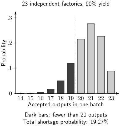
Calculated factory example, not device data. The mean of 20.7 accepted states exceeds the request for 20, yet about 19.3% of batches fall short when no stored states are available. Dark bars mark shortages; the dashed line separates fewer than 20 outputs from sufficient batches. Very small probabilities below 14 outputs are omitted from the plotted range, but included in the stated probability.

Prefilling a buffer, adding factories, changing the schedule, or pausing safely can reduce the consequence. A pause increases memory exposure; a discarded resource can waste preparation time. Factory acceptance is also distinct from the error probability of an accepted state. Correlated rejected or faulty outputs invalidate the independent binomial model. Magic-state distillation and resource estimation develop those separate issues.

Classical processing has throughput and latency requirements

If $N_c$ checks produce $b$ bits per cycle of duration $\tau_c$, the raw acquisition rate is $N_cb/\tau_c$. One million checks with one bit every microsecond already produce $10^{12}$ bits per second, before extra confidence values or leakage flags. Distributed processing can reduce long-distance transport, but the required measurements still have to be handled.

Throughput asks whether processing can keep up with sustained arrivals. Latency asks how long a particular decision takes. A pipelined decoder may have latency longer than a QEC cycle while processing one new cycle’s work each cycle. Conversely, a fast average computation can have long tails during rare difficult inputs. Parallel window decoding addresses such scheduling constraints while reconciling overlapping syndrome regions. Skoric et al. (2023)

Many inferred Pauli corrections can be tracked in a classical Pauli frame instead of being applied immediately. A deadline arises when the next operation or interpretation actually depends on the pending result. Its location depends on the gate protocol and what can be deferred; it is not automatically every cycle or every code deformation. Decoding and real-time control explains the distinction.

If each of $M$ critical decisions has miss probability at most $q$, the union bound limits the probability of any missed deadline by $Mq$. A miss need not be a wrong answer if the machine can pause safely; then count extra runtime and memory faults. The response to a late result is part of the physical model.

Acceptance and correctness answer different questions

For independent fixed-duration attempts taking time $T$, let $a$ be the probability that a result is accepted and $q$ the probability that an accepted result is correct. The mean time to an accepted answer is $T/a$. Its conditional correctness is still $q$.

The ratio $T/(aq)$ is cost per correct accepted output in a long-run yield calculation. It is also the mean waiting time to the first correct accepted output as a mathematical event. It is an operational stopping time only if correctness can be recognized. An unknown quantum state or a difficult computational answer does not generally provide that label for free.

For instance, two-hour runs with $a=0.4$ and $q=0.99$ take five hours on average to deliver an accepted answer. Without an additional verifier, the user receives a 99%-correct answer, not a guaranteed correct answer after a known 5.05 hours. Algorithmic benchmarking explains task-specific success and retry models.

Exercises

1. Allocate a failure allowance

A model contains $4\times10^8$ Clifford locations, $2\times10^7$ injected resources and $10^6$ final measurements. Allocate allowances 0.004, 0.004 and 0.002, respectively. What uniform probability bound is sufficient within each class?

Solution

Divide each allowance by its number of opportunities:

$$\begin{aligned} p_C&\leq10^{-11},\\ p_T&\leq2\times10^{-10},\\ p_M&\leq2\times10^{-9}. \end{aligned}$$

Their weighted sum is 0.01. The bound does not require independent failure events, but every relevant failure source must be covered. Additional preparation or control failures need their own allowance or inclusion in these bounds.

2. Find a conditional distance

In $p_L=0.1(0.1)^{(d+1)/2}$, find the smallest odd distance reaching $10^{-12}$.

Solution

The condition is $1+(d+1)/2\geq12$, giving $d\geq21$. Distance 19 gives $10^{-11}$, while distance 21 gives $10^{-12}$. This is conditional on the fitted law and is not a guarantee for a different logical operation or a noise model with an error floor.

3. Size the data path

There are $1.5\times10^6$ check records every $800\,\mathrm{ns}$, each containing two bytes. Can a sustained $3.0\,\mathrm{TB/s}$ pipeline carry them without compression? Use decimal units.

Solution

Each cycle produces three million bytes. Dividing by $8\times10^{-7}$ seconds gives $3.75\,\mathrm{TB/s}$. The input exceeds the service capacity, so unprocessed data accumulate during sustained operation. A finite buffer delays the overflow but does not fix the long-run mismatch.

4. Mean supply and batch shortages

Each factory succeeds with probability 0.9 every 200 cycles. A calculation consumes an average of one resource per ten cycles. Find the smallest factory count meeting the mean-rate condition. Does it guarantee 20 outputs at the first batch boundary?

Solution

The condition $0.9F/200\geq0.1$ gives $F\geq22.22\ldots$, hence at least 23 factories. No deadline guarantee follows: for independent attempts and an empty initial buffer, the calculation above gives a 19.27% probability of fewer than 20 outputs. The mean is sufficient only as an average capacity check; buffering and the permitted stall probability still matter.

5. Compare the same memory task

An encoded memory succeeds with probability 0.995 after two milliseconds. A physical reference succeeds with probability 0.990 after four milliseconds. Has the encoded memory beaten that reference?

Solution

Not on the same storage task. The elapsed times differ. Compare both channels at the requested duration, with compatible input states, preparation, readout, acceptance and uncertainty. Extrapolating either probability to another duration requires a model.

6. When can a retry stop?

Use the two-hour, 40%-accepted, 99%-correct example. What changes if an ideal external check recognizes every correct and incorrect accepted answer at negligible cost?

Solution

Without the extra check, stopping at acceptance takes five hours on average and leaves 1% conditional error. With it, the recognized success probability per run is $0.4\times0.99=0.396$. Repeating until recognized success then takes

$$\frac{2\,\mathrm h}{0.396}\approx5.05\,\mathrm h$$

on average. The ideal verifier is an additional assumption, often unavailable for the task of interest.

7. Diagnose an error floor

Suppose $p_L(d)=0.08(0.45)^{(d+1)/2}+2\times10^{-7}$. Can increasing distance alone reach $10^{-9}$?

Solution

No. The distance-dependent term tends to zero, leaving a floor 200 times the target. The design must reduce or correct the process represented by that term, or change the target. The formula alone does not identify its physical cause or prove that it is fundamental.

8. Interpret a memory-resource comparison

A simulated high-rate code needs one tenth the memory qubits of a surface-code model at the same logical-memory target. Does it follow that a complete algorithm needs one tenth the hardware?

Solution

No. The result concerns the compared memory circuits under the specified noise, connectivity and decoding assumptions. Logical gates, factories, routing, selective access and control can change the total. It is a useful component-level comparison that must be extended to the compiled workload before drawing that larger conclusion.

References

• M. E. Beverland et al., “Assessing requirements to scale to practical quantum advantage,” arXiv:2211.07629 (2022). Author preprint.
• S. Bravyi and A. Kitaev, “Universal quantum computation with ideal Clifford gates and noisy ancillas,” Physical Review A 71, 022316 (2005). doi:10.1103/PhysRevA.71.022316.
• B. Eastin and E. Knill, “Restrictions on transversal encoded quantum gate sets,” Physical Review Letters 102, 110502 (2009). doi:10.1103/PhysRevLett.102.110502.
• A. G. Fowler, M. Mariantoni, J. M. Martinis, and A. N. Cleland, “Surface codes: Towards practical large-scale quantum computation,” Physical Review A 86, 032324 (2012). doi:10.1103/PhysRevA.86.032324.
• L. Skoric, D. E. Browne, K. M. Barnes, N. I. Gillespie, and E. T. Campbell, “Parallel window decoding enables scalable fault tolerant quantum computation,” Nature Communications 14, 7040 (2023). doi:10.1038/s41467-023-42482-1.