Error-Correction Case Studies

Quantum error correction succeeds when the complete encoding, measurement, decoding, and recovery procedure preserves information better than a specified alternative. Detecting an error is only one part of that task. These case studies connect a small syndrome example to surface-code memories, oscillator encodings, and logical operations, emphasizing what each experiment actually measures.

Helpful background. Why quantum error correction is possible explains how errors can be learned without measuring the logical state. Stabilizers and the surface code introduce check operators and code distance. Logical benchmarking develops the measurement protocols used here.

Reading a syndrome without reading the qubit

The three-qubit repetition code maps an unknown state to

$$|\psi_L\rangle=\alpha|000\rangle+\beta|111\rangle.$$

Its checks are $S_1=Z_1Z_2$ and $S_2=Z_2Z_3$. A parity measurement learns whether adjacent bits agree, while leaving the amplitudes $\alpha,\beta$ undisclosed. Under the candidate error set $\{I,X_1,X_2,X_3\}$, the outcomes identify the error:

Error	$S_1$	$S_2$
$I$	$+1$	$+1$
$X_1$	$-1$	$+1$
$X_2$	$-1$	$-1$
$X_3$	$+1$	$-1$

This code can preserve an arbitrary superposition against a single bit flip. It cannot correct arbitrary single-qubit noise: $Z_1$ commutes with both checks and changes the logical relative phase. Calling the code purely classical misses the first fact; calling it protection against arbitrary errors misses the second.

Real check measurements also fail. Let $s_j(t)$ be the reported parity bit for check $j$ in round $t$, with zero meaning eigenvalue $+1$. A detection event records a change,

$$\delta_j(t)=s_j(t)\oplus s_j(t-1).$$

If $X_2$ occurs between rounds, both checks change together. If one check is merely misreported for one round, that check changes entering and leaving the bad sample. A decoder uses these patterns and a noise model to infer a recovery; the pattern need not identify a unique physical history.

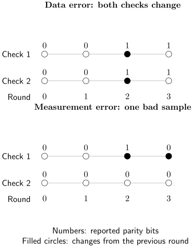
Filled circles mark detection events. Top: an $X_2$ data error changes both checks at round 2. Bottom: only check 1 is misreported in round 2, producing events at rounds 2 and 3. Initial parity is known; actual circuits also need final boundary information and can produce more complicated patterns.

Correction need not mean applying an extra physical gate immediately. A Pauli frame records a known correction in software and uses it when interpreting later measurements or controls. Offline reinterpretation of a final measurement tests the memory and decoder. Supplying the frame during a continuing computation additionally tests the timing of classical processing.

A repetition-code experiment

Google Quantum AI’s 2021 superconducting experiment used repetition codes up to distance 11, with 21 total data and measurement qubits and as many as 50 rounds. In the phase-flip family, logical error per round fell from $8.7\times10^{-3}$ for five total qubits to $6.7\times10^{-5}$ for 21. This tested suppression of the protected error sector, not simultaneous protection against both bit and phase errors. Data near rare high-energy disturbances were excluded to study typical operation; those disturbances affected less than $0.5\%$ of the data. The exclusion matters when applying the result to uninterrupted operation. Google Quantum AI (2021)

What a logical memory lifetime means

A logical memory must preserve more than the population of $|0_L\rangle$. For example, a random logical $Z$ error leaves that state intact while damaging $|+_L\rangle$. Preparing states along several Bloch-sphere axes reveals this difference. Six cardinal-state survival measurements can determine an average fidelity, but do not by themselves determine every entry of a channel’s process matrix.

One common model assumes that a chosen binary logical observable flips independently with probability $e$ per cycle. After $r$ cycles,

$$P_{\rm wrong}(r)=\frac{1-(1-2e)^r}{2}.$$

Two flips can cancel in the final outcome. Consequently this endpoint probability differs from the probability that any logical flip occurred. It approaches one half rather than one. The derivation and preparation/readout corrections are given in logical benchmarking.

For cycle duration $\tau_c$ and $0<e<1/2$, the corresponding exponential contrast lifetime is

$$T_C=-\frac{\tau_c}{\ln(1-2e)} \simeq\frac{\tau_c}{2e}.$$

The factor of two matters: the effective continuous-time flip rate is $\gamma=-\ln(1-2e)/(2\tau_c)$, approximately $e/\tau_c$, whereas contrast decays at rate $2\gamma$. An experimentally quoted lifetime may instead average several axes or use a process-fidelity fit. Use its stated definition before converting it into an error rate.

Break-even compares a logical lifetime with a named reference, $G=T_L/T_{\rm ref}$. The same encoding without correction tests whether the correction loop helps. A physical qubit or an uncorrected oscillator encoding tests a different comparison. Match elapsed time, prepared states, active controls, discarded trials, and treatment of preparation and measurement errors. A ratio against one reference does not automatically apply to another.

Increasing surface-code distance

A larger surface code uses more data and measurement qubits to make a logical error require a larger damaging pattern of faults. More qubits also introduce more places for faults. The competition produces a threshold: increasing distance helps only in a sufficiently favorable noise regime for the circuit and decoder.

For matched odd distances, an empirical suppression factor is

$$\Lambda_d=\frac{e_d}{e_{d+2}}.$$

A value above one means the larger tested code had a smaller error in that comparison. It is not a universal physical-error threshold, and one pair of sizes cannot guarantee the same reduction indefinitely. Leakage, correlations, changing hardware quality, and finite-size effects can change the trend.

The Google surface-code study published in 2025 reported a distance-7 memory using 101 qubits and logical error $0.143\%\pm0.003\%$ per cycle. Its distance-step suppression factor was $2.14\pm0.02$. The reported logical lifetime was $291\pm6\,\mu\mathrm{s}$, compared with $119\pm13\,\mu\mathrm{s}$ for its best constituent physical reference, a gain of $2.4\pm0.3$. A distance-5 implementation used real-time decoding with mean latency $63\,\mu\mathrm{s}$ for $1.1\,\mu\mathrm{s}$ cycles. These are distinct demonstrations of size suppression, memory gain, and live classical processing. Google Quantum AI and Collaborators (2025)

Latency longer than one cycle is compatible with a pipeline: several rounds can be in processing simultaneously. Sustained throughput must keep up with incoming rounds, and a dependent operation must receive the needed frame before its deadline. Mean latency alone does not establish either property.

The same study used long repetition codes to probe rare correlated disturbances. Its corrected Figure 3a concerns repetition-code distance, not surface-code distance; the 2026 correction fixes that labeling. A floor inferred from this diagnostic should not be relabeled as a measured surface-code floor. The surface-code result itself concerns memory; protected gates and non-Clifford resources require additional tests.

Oscillator codes and the choice of reference

An oscillator has many levels in which to store redundancy. This can reduce the number of separate storage elements, while still requiring ancillary qubits, control pulses, readout, and reset. The relevant unit is the complete memory module, not an isolated oscillator without its correction apparatus.

GKP codes encode a qubit in a grid-like phase-space structure. Finite-energy implementations have approximate grid peaks, and repeated correction suppresses small displacement errors. Sivak and colleagues demonstrated a stabilized superconducting GKP memory with coherence gain $2.27\pm0.07$ over the best imperfect component in their comparison. This was a substantial memory improvement in one module; it was not a measurement of an increasing-distance family. Sivak et al. (2023)

Binomial codes use selected number-state superpositions. Ni and colleagues used

$$\begin{aligned} |0_L\rangle&=(|0\rangle+|4\rangle)/\sqrt2,\\ |1_L\rangle&=|2\rangle. \end{aligned}$$

A single photon loss maps these basis states to $\sqrt2|3\rangle$ and $\sqrt2|1\rangle$. Equal norms are crucial: learning that a loss occurred does not reveal which logical basis state was present. The experiment repeatedly extracted a loss syndrome and applied feedback, exceeding its physical-memory comparison by about $16\%$. That reference was a qubit in the cavity’s lowest two Fock states, not the cavity’s raw energy-decay time. Ni et al. (2023)

Photon loss is not the whole evolution. The no-jump attenuation also changes number-state amplitudes, while missed multiple losses, ancilla faults, and recovery errors limit performance. The code and its correction cadence must address the actual channel. A gain for one oscillator encoding and a gain for another need not rank the two architectures: their reference memories and lifetime definitions can differ.

From storage to continuing logical operations

The neutral-atom experiment of Bluvstein and colleagues illustrates why separate parts of a paper must be read separately. Its four-round surface-code benchmark found a $2.14(13)$ reduction in error per round from distance 3 to 5 using loss information and machine-learning decoding, without postselection in that comparison. Other experiments implemented logical entangling operations, code teleportation, and qubit reuse. The reuse circuits supported dozens of logical qubits and hundreds of logical teleportations; they were not limited to the four-round memory benchmark. Bluvstein et al. (2026)

These results connect protection with repeated operations and entropy removal. They do not make the surface-code suppression factor a measured error rate for every gate or every deeper circuit in the paper. To assess a computation, follow its own encoding, circuit, decoding, acceptance, and output statistics. Fault-tolerant gates explains fault propagation; lattice surgery and magic-state distillation develop specific ways to perform logical operations.

Exercises

1. Two faults imitate one

The repetition-code syndrome is $(-1,+1)$. Why can the one-fault decoder choose $X_1$, yet fail when the actual fault was $X_2X_3$?

Solution

Both operators anticommute with $S_1$ and commute with $S_2$. Applying the inferred recovery $X_1$ after $X_2X_3$ leaves $X_1X_2X_3=\overline X$, a logical flip. The measured checks specify a syndrome class; the noise assumptions determine which member the decoder favors.

2. A bad measurement round

One check reports parity bits $0,1,0,0$, including a known initial value. Find its detection-event bits and explain the simplest fault history.

Solution

Adjacent XORs give $1,1,0$. A single erroneous report in the second entry creates two adjacent-time events. A persistent data error would instead keep the parity changed until another fault, recovery, or final boundary. More complicated fault combinations can reproduce the same observed history.

3. Infer the flip probability

For $P_{\rm wrong}=0.18$ after 20 independent identical-flip cycles, find $e$ and compare with $0.18/20$.

Solution

$$e=\frac{1-0.64^{1/20}}2\approx0.01103.$$

The linear estimate is $0.009$, which underestimates $e$ because two or more flips can restore the final parity. The inversion assumes stationary independent flips and an endpoint probability with preparation and readout treated consistently.

4. Per cycle or per second?

Memory A has $e_A=0.0012$ per $2.5\,\mu\mathrm{s}$ cycle; B has $e_B=0.0007$ per $1.0\,\mu\mathrm{s}$ cycle. Compare their approximate flip rates and contrast lifetimes.

Solution

B has less error per cycle. But the approximate rates are $\gamma_A=480\,\mathrm{s}^{-1}$ and $\gamma_B=700\,\mathrm{s}^{-1}$. Thus

$$\begin{aligned} T_{C,A}&\simeq1.04\,\mathrm{ms},\\ T_{C,B}&\simeq0.714\,\mathrm{ms}. \end{aligned}$$

A preserves the chosen contrast longer in elapsed time under this model. The result follows from $T_C\simeq1/(2\gamma)$, not $1/\gamma$.

5. A burst floor

Ordinary operation fails with probability $10^{-5}$ per trial. A burst occurs with probability $10^{-4}$ per trial and then causes failure with probability $1/2$. Find the total failure probability and its limit if ordinary errors are suppressed further.

Solution

$$\begin{aligned} P_{\rm fail}&=(1-10^{-4})10^{-5}+10^{-4}/2\\ &=5.9999\times10^{-5}. \end{aligned}$$

The limiting value is $5\times10^{-5}$ if the burst process stays unchanged. Removing burst trials estimates the conditional ordinary-error probability, not this total probability. A trial here is the entire stated storage experiment; the burst probability is not automatically a per-cycle rate.

6. The uncertainty in a lifetime gain

Let $T_L=230\pm8\,\mu\mathrm{s}$ and $T_R=205\pm7\,\mu\mathrm{s}$, with independent approximately Gaussian standard uncertainties. Estimate $G$ and an approximate 95% interval.

Solution

First-order propagation gives

$$\begin{aligned} G&=230/205=1.1220\ldots,\\ \sigma_G&\simeq G\sqrt{(8/230)^2+(7/205)^2}\\ &=0.0547\ldots. \end{aligned}$$

The approximate interval $G\pm1.96\sigma_G$ is $[1.015,1.229]$. It narrowly excludes one under the stated assumptions. Shared calibration errors require a covariance term; fitted uncertainties do not cover an unmatched state ensemble or an unsuitable reference.

7. Why equal loss amplitudes matter

Apply the oscillator annihilation operator to both binomial basis states above. Compare with the alternative encoding $|0'_L\rangle=|1\rangle$, $|1'_L\rangle=|3\rangle$. Does a detected loss preserve arbitrary logical amplitudes equally in both encodings?

Solution

For the binomial code, write $|\psi_L\rangle=\alpha|0_L\rangle+\beta|1_L\rangle$. Then

$$a|\psi_L\rangle=\sqrt2(\alpha|3\rangle+\beta|1\rangle).$$

After normalization, the amplitudes are unchanged in the error basis. In the alternative code the result is $\alpha|0\rangle+\sqrt3\beta|2\rangle$, with squared norm $|\alpha|^2+3|\beta|^2$. The loss probability reveals logical-state information. Orthogonal output states alone do not make this loss correctable by a state-independent deterministic recovery.

8. A delayed decoder

A decoder pipeline accepts one new syndrome round every microsecond and returns each result $60\,\mu\mathrm{s}$ later. A dependent operation needs the most recent round’s frame within $10\,\mu\mathrm{s}$. Can throughput be adequate while the operation still has to wait?

Solution

Yes. A pipeline can have roughly 60 rounds in flight without an ever-growing queue if it sustains the input rate. Its $60\,\mu\mathrm{s}$ latency nevertheless misses the $10\,\mu\mathrm{s}$ deadline. The operation must wait, be rescheduled, or use a justified alternative protocol. Average throughput and decision latency answer different questions.

References

• D. Bluvstein et al., “A fault-tolerant neutral-atom architecture for universal quantum computation,” Nature 649, 39–46 (2026). doi:10.1038/s41586-025-09848-5.
• Google Quantum AI, “Exponential suppression of bit or phase errors with cyclic error correction,” Nature 595, 383–387 (2021). doi:10.1038/s41586-021-03588-y.
• Google Quantum AI and Collaborators, “Quantum error correction below the surface code threshold,” Nature 638, 920–926 (2025). doi:10.1038/s41586-024-08449-y. Figure-label correction: Nature 653, E5 (2026), doi:10.1038/s41586-026-10559-8.
• Z. Ni et al., “Beating the break-even point with a discrete-variable-encoded logical qubit,” Nature 616, 56–60 (2023). doi:10.1038/s41586-023-05784-4.
• V. V. Sivak et al., “Real-time quantum error correction beyond break-even,” Nature 616, 50–55 (2023). doi:10.1038/s41586-023-05782-6.