Optimization Case Studies

An optimization algorithm searches for a good solution subject to constraints. A quantum device usually sees an encoded energy function instead. The case studies below explain when these are the same problem, what a measured improvement means, and why success on one family of instances need not transfer to another.

Required background. Optimization algorithms introduces objective values, constraints and solution guarantees. Helpful background. QAOA and variational algorithms explain parameterized circuits; Grover search explains query speedups. Algorithmic benchmarking develops comparisons at a fixed success target.

A penalty must enforce the intended constraint

Consider two adjacent vertices with weights 1 and 2. An independent set may select either vertex, but not both. Write $x_i=1$ when vertex $i$ is selected. A quadratic unconstrained binary objective is

$$E(x_1,x_2)=-x_1-2x_2+\lambda x_1x_2.$$

The first two terms reward selected weight; the last penalizes the forbidden pair. Its four energies are

$$\begin{aligned} E(0,0)&=0,&E(1,0)&=-1,\\ E(0,1)&=-2,&E(1,1)&=-3+\lambda. \end{aligned}$$

The correct answer is $(0,1)$, but it is the unique ground state only when $\lambda>1$. At $\lambda=1$, an invalid answer ties with it. Minimizing the implemented energy is therefore insufficient unless the encoding has the right ground states.

Making $\lambda$ arbitrarily large creates another difficulty on hardware with a limited coefficient range. As a simple model, divide every coefficient by $\max(2,\lambda)$ so that the largest magnitude is one. The energy difference between the two nonempty feasible sets becomes $1/\max(2,\lambda)$. It decreases at large penalty even though the mathematical minimizer is unchanged. Finite coefficient precision or noise may then obscure which feasible answer is better.

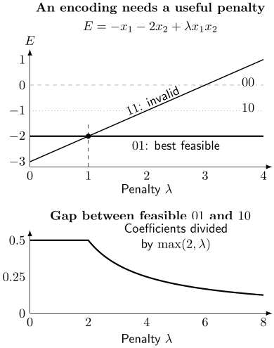
Exact energies for the two-variable example. The lower panel assumes uniform normalization by the largest QUBO coefficient. It illustrates a tradeoff between suppressing invalid answers and resolving feasible ones; it is not a universal hardware-noise threshold.

A general sufficient bound makes the assumptions explicit. Suppose $C(x)\ge L$ for all candidates, a known feasible candidate has cost at most $U$, and every positive constraint penalty obeys $P(x)\ge p_{\min}>0$. Then minimizing $C+\lambda P$ has only feasible global minimizers if

$$\lambda>\frac{U-L}{p_{\min}}.$$

Indeed, every infeasible energy exceeds $L+\lambda p_{\min}>U$. A bound on costs only within the feasible set cannot support this argument: an infeasible candidate might have a much lower unpenalized cost. The bound is sufficient, and can be conservative.

QAOA: a better mean is not always a better chance of success

For a maximization problem, QAOA often optimizes the average score $\langle C\rangle$ of its output distribution. An application might instead require a score above a threshold, or the exact optimum. These objectives differ. A sampler returning score 8 every time has a better mean than one returning 10 with probability 0.6 and zero otherwise. Only the second sampler can find an optimum of 10.

Harrigan and collaborators (2021) ran QAOA for graph problems on a superconducting processor. Their comparison included problems compatible with the hardware connectivity and problems requiring additional routing. Some deep circuits produced better samples than uniform random sampling, while efficient classical methods still outperformed the demonstrated results. The important lesson is how graph compilation and noise affect the distribution of solutions, not just the abstract number of QAOA layers.

Shaydulin and collaborators (2024) studied low-autocorrelation binary sequences, where a bit string is chosen to suppress correlations with shifted copies of itself. Noiseless numerical simulations reached 40 qubits and suggested favorable empirical scaling relative to exact branch-and-bound solvers. The work also considered combination with quantum minimum finding and demonstrated smaller trapped-ion circuits with error detection. The simulated scaling, the coherent algorithmic construction and the executed device experiments are distinct results. Fitting a scaling curve does not remove error correction, circuit construction or repetition costs from a future implementation.

Lu and collaborators (2026) illustrate a useful preprocessing idea for positive one-in-three SAT: each clause asks for exactly one of three bits to equal one. Every valid assignment also obeys an odd-parity equation. For a consistent system of $n$ bits and parity rank $r$, the relaxed subspace has $2^{n-r}$ basis strings. The paper combines this reduction with QAOA, includes classical comparisons that use the reduction, and demonstrates 22-variable instances using 13 hardware qubits. The distinction between parity and the original constraint is essential: $111$ has odd parity but does not have exactly one occupied bit. The remaining optimization must still distinguish such strings.

Rydberg independent sets: geometry creates both constraints and structure

Rydberg blockade suppresses simultaneous excitations of sufficiently close atoms. In an idealized graph model, excited atoms represent selected vertices and close pairs represent exclusion edges. Positive detuning rewards excitation, while strong repulsion penalizes adjacent selections. Uniform detuning assigns equal rewards; weighted independent sets generally need site-dependent rewards or a more elaborate encoding.

Ebadi and collaborators (2022) used arrays of up to 289 atoms for maximum independent set instances. Optimized quantum protocols showed favorable performance against the simulated-annealing comparisons used in that study. Finite interactions, long-range tails and the geometry of the graph remain part of the physical problem: a sharp exclusion graph is an approximation to an interacting atom array.

Andrist and collaborators (2023) examined a broader set of classical solvers and graph structures. Quasi-planar instances with Union-Jack-like connectivity could be solved to optimality for thousands of vertices within minutes, and a less restricted simulated-annealing implementation was competitive with the earlier quantum protocols. Less structured or more highly connected instances could be substantially harder. Thus atom count is not a measure of instance difficulty. Geometry can make a problem convenient for a quantum device and simultaneously useful to a classical algorithm.

Annealing: what a selected classical comparison establishes

Denchev and collaborators (2016) designed weak–strong cluster instances to study collective tunneling in a superconducting annealer. They reported large finite-size speedups relative to particular single-core simulated-annealing and quantum-Monte-Carlo implementations. A tunneling mechanism and a favorable comparison against those algorithms are meaningful findings. Neither implies superiority to every classical solver.

Mandrà and collaborators (2016) compared a wider range of methods on this family. Classical approaches exploiting the graph structure changed the performance comparison. This does not erase the physical tunneling question; it changes the computational conclusion. A claim about a mechanism, a claim about one competitor, and a claim about the best available algorithms require different comparisons.

For application instances that do not match a device graph, embedding can add chains of physical qubits, couplings and decoding steps. The resulting answer must be scored in the original problem after decoding. A low physical energy with broken chains need not identify a feasible or high-quality original solution. See quantum annealing for the encoding and dynamics.

Search speedups must include the reversible computation

Grover search can reduce the number of calls to a Boolean predicate. The predicate must nevertheless compute constraints, objective comparisons and any necessary arithmetic reversibly, then uncompute temporary data. Searching a flat space also discards the pruning that can make a classical instance easy.

Campbell, Khurana and Montanaro (2019) estimated fault-tolerant resources for search and backtracking on satisfiability and graph-coloring problems. Their study shows how large circuit and error-correction costs can accompany a favorable query count. Including the classical computation needed for decoding can change the comparison again. Such estimates are conditional calculations, not dates at which a useful machine will exist.

For a particular instance, let $T$ be the number of nodes explored by a classical search tree. Quantum backtracking can offer square-root-type dependence on $T$ under suitable access assumptions, with additional depth and algorithmic factors. The number of leaves alone does not determine $T$ unless the tree shape is constrained. A small query exponent cannot substitute for the cost of reversible branching and bounds.

From success probability to elapsed time

Suppose each independent run succeeds with probability $p$ at a fixed, verified quality threshold. The number of runs needed for success probability at least $1-\delta$ is

$$R_\delta=\left\lceil \frac{\ln\delta}{\ln(1-p)}\right\rceil.$$

At $p=0.02$, 228 runs give at least 99% success. If each run takes 4 ms and one-time setup takes 0.8 s, the total is 1.712 s. Setup belongs outside the repeated term only if it is actually reused. Correlated failures, drift or an uncertain estimate of $p$ require a richer model; see algorithmic benchmarking for those cases.

Solution quality also needs a meaningful denominator. For a nonnegative maximization objective with true optimum $C^\star$, a feasible value $C$ has ratio $C/C^\star$. A best-known value is not necessarily $C^\star$. If a valid upper bound $B\ge C^\star>0$ is available, then $C/B$ is a lower bound on this ratio. Adding a constant to every objective value preserves the optimization problem but changes the numerical ratio, so the objective normalization must be fixed before interpreting it.

Exercises

1. The penalty threshold

Enumerate the two-variable example at $\lambda=0.5$, $1$ and $1.5$. Which values ensure that every ground state is feasible?

Solution

The first three energies are always $0,-1,-2$. The invalid state’s energy is respectively $-2.5,-2,-1.5$. It wins at 0.5, ties at 1, and loses at 1.5. Only 1.5 guarantees feasibility of every minimizing answer. A tie cannot be dismissed unless a separate rule is guaranteed to resolve it correctly.

2. A bound that applies outside the feasible set

All feasible costs lie between 0 and 20, and every violation has penalty at least one. Does $\lambda=21$ ensure feasibility? What changes if a global bound $C\ge-5$ and a known feasible cost $U=20$ are supplied?

Solution

The first information is insufficient. An infeasible candidate with $C=-100$ and $P=1$ still has energy $-79$. With the additional global bound, the sufficient condition is $\lambda>25$. At equality, an infeasible point with cost $-5$ can tie a feasible point of cost 20. The strict inequality removes this possibility.

3. Rescaling the useful gap

In the two-vertex model, compare the gap between the two nonempty feasible states after coefficient normalization at $\lambda=1.5$ and $\lambda=20$.

Solution

The unscaled gap is one. The normalized gaps are $1/2=0.5$ and $1/20=0.05$. Both penalties select the right mathematical minimizer, but the second encoding makes this feasible distinction ten times smaller. Whether that matters experimentally depends on coefficient precision and the physical error model.

4. Mean score and optimum probability

Compare the two samplers with scores 8 always, and 10 with probability 0.6 or zero otherwise. How many independent calls to the second give at least 99% probability of seeing 10?

Solution

Their means are 8 and 6. The first has zero exact-success probability, while the second needs

$$R=\left\lceil\frac{\ln0.01}{\ln0.4}\right\rceil=6.$$

Five calls give $1-0.4^5=0.98976$, below 99%; six give $0.995904$. The preferred distribution therefore depends on the requested output.

5. Parity is a relaxation

Two identical clauses require exactly one of $x_1,x_2,x_3$ to be one. How many assignments survive their parity equations, and how many satisfy the clauses?

Solution

The duplicate parity equations have rank one, not two. Four strings survive: $100,010,001,111$. Only the first three satisfy exactly-one. Counting clauses would incorrectly predict $2^{3-2}=2$ survivors; the rank formula gives $2^{3-1}=4$.

6. A scaling crossover

Illustrative runtime models are $T_Q=10^6(1.008)^n$ and $T_C=(1.013)^n$ in the same units. At what real-valued $n$ do they cross?

Solution

Taking logarithms gives

$$n=\frac{\ln10^6}{\ln(1.013/1.008)} \approx2792.11.$$

The quantum model first becomes smaller at integer $n=2793$. Its better exponent is offset by a large prefactor over a long range. Extrapolation that far also requires justification that both fitted forms remain valid.

7. Ratios and bounds

A feasible maximization score is 92, the best-known score is 106, and a valid upper bound is 110. What ratio is guaranteed? How does adding 100 to every score change it?

Solution

The guaranteed ratio is at least $92/110\approx0.83636$. The value $92/106$ compares two feasible scores but need not be the ratio to the optimum. After the shift, the guaranteed ratio becomes $192/210\approx0.91429$, although the candidate ordering and optimal strings have not changed. Approximation ratios are properties of a specified objective normalization.

8. Leaves and nodes

A perfect binary tree has $2^{30}$ leaves. How many total nodes does it have? Why does its leaf count not determine the node count of a general tree with chains of single-child nodes?

Solution

The perfect tree has

$$T=1+2+\cdots+2^{30}=2^{31}-1.$$

Inserting arbitrarily many single-child nodes leaves the leaf count unchanged while increasing $T$. Even $\sqrt T$ specifies only one factor in a quantum-backtracking estimate; depth, access and reversible-operation costs remain.

9. Repetitions and setup

Verify the 1.712 s example. What would change if the 0.8 s preparation had to be repeated for every run?

Solution

The failure probabilities at 227 and 228 calls are approximately 0.01019 and 0.00999. Thus 228 is minimal, and reusable setup gives $0.8+228(0.004)=1.712$ s. Repeated preparation instead gives $228(0.804)=183.312$ s. The same success probability can correspond to very different elapsed times.

References

• Andrist, R. S., et al. “Hardness of the maximum independent set problem on unit-disk graphs and prospects for quantum speedups.” Physical Review Research 5, 043277 (2023). doi:10.1103/PhysRevResearch.5.043277.
• Campbell, E., Khurana, A., and Montanaro, A. “Applying quantum algorithms to constraint satisfaction problems.” Quantum 3, 167 (2019). doi:10.22331/q-2019-07-18-167.
• Denchev, V. S., et al. “What is the computational value of finite-range tunneling?” Physical Review X 6, 031015 (2016). doi:10.1103/PhysRevX.6.031015.
• Ebadi, S., et al. “Quantum optimization of maximum independent set using Rydberg atom arrays.” Science 376, 1209–1215 (2022). doi:10.1126/science.abo6587.
• Harrigan, M. P., et al. “Quantum approximate optimization of non-planar graph problems on a planar superconducting processor.” Nature Physics 17, 332–336 (2021). doi:10.1038/s41567-020-01105-y.
• Lu, Q., et al. “Evidence of scaling advantage on an NP-complete problem with enhanced quantum solvers.” Nature Computational Science 6, 882–893 (2026). doi:10.1038/s43588-026-01007-8.
• Mandrà, S., Zhu, Z., Wang, W., Perdomo-Ortiz, A., and Katzgraber, H. G. “Strengths and weaknesses of weak–strong cluster problems: A detailed overview of state-of-the-art classical heuristics versus quantum approaches.” Physical Review A 94, 022337 (2016). doi:10.1103/PhysRevA.94.022337.
• Shaydulin, R., et al. “Evidence of scaling advantage for the quantum approximate optimization algorithm on a classically intractable problem.” Science Advances 10, eadm6761 (2024). doi:10.1126/sciadv.adm6761.