Quantum Annealing

Quantum annealing uses a changing quantum Hamiltonian to produce candidate solutions, often low-cost bit strings. A driver initially mixes configurations; the problem Hamiltonian favors the desired answers. Coherent transitions, thermal relaxation and the measurement process can all influence the returned distribution. Unlike ideal adiabatic quantum computation, an annealing protocol may deliberately use fast changes, pauses or reversals. Its usefulness depends on the measured answers and total cost, not merely on whether a quantum mechanism is present.

Helpful background. Adiabatic quantum computation explains Hamiltonian encodings and gaps. Thermal master equations explains when thermal transition rates provide a valid dynamical model.

Driver and problem Hamiltonians

With $Z|0\rangle=|0\rangle$ and $Z|1\rangle=-|1\rangle$, bits and spin values obey

$$s_i=(-1)^{x_i},\qquad x_i=\frac{1-s_i}{2}.$$

A two-local Ising objective has the form

$$H_{\mathrm P}=cI+\sum_i h_iZ_i+\sum_{i<j}J_{ij}Z_iZ_j.$$

The common transverse driver $H_{\mathrm D}=-\sum_i\Gamma_iX_i$, with $\Gamma_i>0$, has product ground state $|+\rangle^{\otimes n}$. A schedule can use

$$H(t)=A(t)H_{\mathrm D}+B(t)H_{\mathrm P}+H_{\mathrm{cat}}(t).$$

Here $H_{\mathrm{cat}}$ denotes any additional control terms. If the component Hamiltonians have energy units, $A$ and $B$ are dimensionless; other conventions must specify where the energy scale sits. Nonuniform or interacting drivers can change both preparation difficulty and the accessible dynamics.

For a decoder $D$ and objective $C$, the diagonal relation

$$H_{\mathrm P}=\sum_z [aC(D(z))+b]|z\rangle\langle z|, \qquad a>0,$$

preserves the ordering of decoded costs. Increasing $a$ also changes physical gaps, thermal ratios and usually transition rates. A uniform scalar offset $bI$ cancels from the normalized Gibbs state and contributes only a common phase to isolated evolution. Constraint penalties and chain couplings must fit the available coefficient range; making them stronger may require reducing all other physical energy scales.

Define success after decoding. If $\mathcal A$ is the accepted set of answers, then physical string $z$ succeeds when $D(z)\in\mathcal A$. Several ground strings may all be valid, and broken-chain repair or rejection changes the returned distribution.

A schedule determines a process

A forward anneal usually reduces the relative driver strength and increases the problem strength. A pause holds selected coefficients fixed. A reverse anneal starts from a specified seed near the problem endpoint, moves toward a stronger driver and returns. A quench idealizes a rapid change; finite control bandwidth determines how well that idealization applies.

The initial state, full schedule and dynamics are needed to predict samples. For a terminal state $\rho(T)$ and measurement effects $M_y$,

$$p_T(y)=\operatorname{Tr}[M_y\rho(T)], \qquad p_{\mathrm{acc}}=\sum_{y:D(y)\in\mathcal A}p_T(y).$$

If a classical readout channel $R(y|z)$ follows an ideal computational-basis measurement, then $p_{\mathrm{obs}}(y)=\sum_zR(y|z)p_T(z)$, and acceptance must use the actually reported outcomes.

Closed evolution follows $i\hbar\dot\psi=H(t)\psi$. It has no bath temperature, although the initial state may be thermal. For an open system,

$$\rho_S(t)=\operatorname{Tr}_E[U_{SE}(t)\rho_{SE}(0)U_{SE}(t)^\dagger].$$

A fixed initial environment uncorrelated with arbitrary system inputs defines a channel on those inputs. With correlated preparations, the reduced evolution cannot automatically be represented by one channel on every possible system state.

A master equation such as

$$\dot\rho=-\frac{i}{\hbar}[H(t),\rho]+\mathcal D_t(\rho)$$

requires specified coupling operators, rates and approximation conditions. Weak-coupling thermal generators for slowly varying Hamiltonians have additional time-scale and secular requirements, as developed by Albash and colleagues. A local dissipator may fail to preserve the Gibbs state of an interacting Hamiltonian. Fast driving, strong coupling or memory can invalidate an instantaneous thermal description.

Coherent example: longer can be worse

Set $\hbar=1$. Prepare the ground state $|+\rangle$ of $H_{\mathrm D}=-X/2$, quench to $H_{\mathrm M}=-(X+Z)/2$, hold for time $\tau$, then quench to $H_{\mathrm P}=-Z/2$ and measure. Ideal zero-duration quenches leave the state unchanged at each switch. During the pulse,

$$\begin{aligned} U_{\mathrm M}(\tau)&=\cos(\tau/\sqrt2)I +i\sin(\tau/\sqrt2)\frac{X+Z}{\sqrt2},\\ |\psi(\tau)\rangle&=\cos(\tau/\sqrt2)|+\rangle +i\sin(\tau/\sqrt2)|0\rangle. \end{aligned}$$

The endpoint ground-state probability and energy are

$$p_0(\tau)=\frac{3-\cos(\sqrt2\tau)}4, \qquad p_1=1-p_0, \qquad \langle H_{\mathrm P}\rangle=\frac12-p_0.$$

Dwell time $\tau$	Ground probability $p_0$	Mean final energy
$0$	$1/2$	$0$
$\pi/(2\sqrt2)$	$3/4$	$-1/4$
$\pi/\sqrt2$	$1$	$-1/2$
$3\pi/(2\sqrt2)$	$3/4$	$-1/4$
$\sqrt2\pi$	$1/2$	$0$

The probability returns to $1/2$ after a longer dwell. This is coherent interference, not relaxation to a thermal state or an application of an adiabatic theorem. A subsequent closed dwell under $H_{\mathrm P}$ changes phases but leaves these measurement probabilities unchanged.

Thermal relaxation and incomplete equilibration

For a fixed two-level energy basis with energies $0$ and $\Delta$, let $p_e$ be the excited-state population. Upward and downward rates give

$$\dot p_e=\Gamma_\uparrow(1-p_e)-\Gamma_\downarrow p_e =-\gamma(p_e-q),$$

where $\gamma=\Gamma_\uparrow+\Gamma_\downarrow$ and $q=\Gamma_\uparrow/\gamma$. Thermal detailed balance requires $\Gamma_\uparrow/\Gamma_\downarrow=e^{-\beta\Delta}$, giving

$$q=\frac1{1+e^{\beta\Delta}}, \qquad p_e(t)=q+[p_e(0)-q]e^{-\gamma t}.$$

The equilibrium population is a destination of this rate law, not a value reached instantly. Relaxation can lower or raise $p_e$, depending on which side of $q$ the incoming state occupies.

For a concrete two-stage model, take $\beta=2$, initial $p_e=1/2$ and parameters $(\Delta,\gamma,t)=(1,1,1)$ followed by $(3,0.1,2)$. The energy basis is fixed, and the instantaneous parameter change is an idealization. Applying the update twice gives

$$\begin{aligned} q_1&=0.1192029220,&p_1&=0.2592903383,\\ q_2&=0.0024726232,&p_2&=0.2127371845. \end{aligned}$$

Thus the actual ground probability is $0.7872628155$, far below the final Gibbs value $0.9975273768$. The second stage removes only the fraction $1-e^{-0.2}\approx0.181269$ of its incoming deviation from $q_2$.

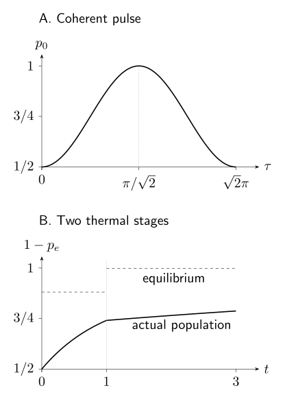
Two explicitly different models. The upper plot is the coherent pulse example; extending the pulse can reduce success. The lower plot follows the thermal rate example; the ground population rises but does not reach the new equilibrium value after the second stage. Neither plot is device data.

For time-dependent rates, define $\Lambda(t)=\int_0^t\gamma(u)\,du$. The exact scalar solution is

$$p_e(T)=e^{-\Lambda(T)}p_e(0) +\int_0^T\gamma(u)q(u)e^{-[\Lambda(T)-\Lambda(u)]}\,du.$$

It remembers the earlier schedule. If the remaining integrated rate $\int_t^T\gamma(u)\,du$ is small, little further relaxation is possible in this model. A useful definition of freeze-out must specify such a kinetic model, observable and tolerance; there is no universal freeze time.

An effective-temperature fit alone cannot establish that mechanism. In the example,

$$\beta_{\mathrm{eff}}=\frac13\ln\!\frac{1-p_2}{p_2} \approx0.4361682,$$

although the bath has $\beta=2$. Every strictly positive two-level diagonal distribution admits a fitted inverse temperature, possibly negative, so the fit is a particularly weak test of equilibration.

There is a useful special case: if the late Hamiltonian is $H(t)=a(t)H_{\mathrm P}+b(t)I$, with $a(t)>0$, and populations equilibrate at $t_*$ then remain frozen in its fixed eigenbasis, fitting them in the final energy units gives $\beta_{\mathrm{eff}}=\beta a(t_*)/a(T)$. Residual transverse terms, later transitions or readout errors can spoil this inference. Amin discusses the quasistatic freeze-out interpretation and its limits.

Stoquasticity, embedding and errors

A Hamiltonian is stoquastic in a specified basis if all off-diagonal entries are real and nonpositive. This may avoid a sign problem in a particular equilibrium representation, but it does not guarantee rapid sampling or easy optimization. Nonstoquasticity, tunneling and entanglement likewise do not establish a speedup. The sign problem and complexity classes explain the separate computational questions.

An embedding represents one logical spin by several physical spins or other controls. Its coupling penalties, coefficient rescaling and broken-chain decoder affect the measured answers. For a spin-reversal gauge $g_i=\pm1$, define $U_g=\prod_{i:g_i=-1}X_i$. Then

$$U_gH(h,J)U_g^\dagger=H(g_ih_i,g_ig_jJ_{ij}), \qquad s_i'=g_is_i.$$

Decode with $s_i=g_is_i'$. The ideal spectrum is unchanged; averaging across gauges may reduce some control biases but is not quantum error correction.

For ideal low-energy accepted states separated from rejected states by $\Delta_{\mathrm{acc}}$, a Hermitian perturbation satisfying $\|\delta H_{\mathrm P}\|<\Delta_{\mathrm{acc}}/2$ preserves a spectral separation. If the error is diagonal in the same computational basis, it also preserves the ordering of those accepted and rejected strings. A general off-diagonal error can rotate the low-energy subspace: a surviving gap alone does not ensure that computational-basis readout returns the same strings. Dynamical and readout errors require additional analysis.

Success probabilities and total time

Mean energy, probability of an exact optimum, feasibility and approximation quality are different statistics. An accepted cost threshold should be fixed before comparing solvers. For known independent per-run $0<p_{\mathrm{acc}}<1$,

$$R_\eta=\left\lceil\frac{\ln(1-\eta)}{\ln(1-p_{\mathrm{acc}})}\right\rceil$$

gives at least one accepted result with probability $\eta$. Recognizing that result requires a checkable target or another justified selection rule. Correlations, drift, varying gauges or uncertainty in an estimated probability require a different statistical treatment.

A simple serial cost model is

$$T_{\mathrm{total},\eta}={}T_{\mathrm{setup}}+T_{\mathrm{program}} +R_\eta(T_{\mathrm{anneal}}+T_{\mathrm{read/reset}} +T_{\mathrm{decode}}+T_{\mathrm{verify}}).$$

This assumes one shared programming step. Reprogramming, multiple gauges, rejected samples and parallel resources must be counted when used. Algorithmic benchmarking explains matched comparisons, and optimization case studies connects them to applications. A successful small example or a short anneal time alone establishes neither favorable scaling nor an advantage.

Exercises

Map a Two-Bit QUBO to an Ising Hamiltonian

Using $x_i=(1-Z_i)/2$, map

$$C=x_1+2x_2-3x_1x_2$$

to a diagonal Ising Hamiltonian. Enumerate the four bit strings, identify the accepted minimum set, and explain which affine changes preserve that set.

Solution

Substitution gives

$$H = \frac34I + \frac14Z_1 - \frac14Z_2 - \frac34Z_1Z_2.$$

In the order $(00,01,10,11)$, the objective values are

$$(0,2,1,0).$$

Thus the accepted set is $\{00,11\}$. Adding a constant and multiplying by a positive number preserve this argmin. They do not preserve every physical statement: a positive scale changes gaps, $\beta H$, control ranges, and generally transition rates.

Apply and Decode a Spin-Reversal Gauge

For

$$H = 0.4Z_1-0.7Z_2+1.2Z_1Z_2,$$

apply the gauge $g=(-1,+1)$, find the transformed Hamiltonian, and decode the transformed ground spin.

Solution

The coefficient rule $h_i'=g_ih_i$, $J_{ij}'=g_ig_jJ_{ij}$ gives

$$H' = -0.4Z_1-0.7Z_2-1.2Z_1Z_2.$$

The original ground spin is $(-,+)$, with energy

$$0.4(-1)-0.7(+1)+1.2(-1)(+1)=-2.3.$$

It maps to the measured transformed spin $(+,+)$. Decoding with $s_i=g_is_i'$ recovers $(-,+)$. The gauge is a unitary relabeling, so the ideal spectrum is invariant; averaging over gauges is not error correction.

Show That Stoquasticity Depends on the Basis

Compare $-X$ with its transform under $Z$. Decide whether each matrix is stoquastic in the computational basis and state what remains invariant.

Solution

In the computational basis,

$$-X = \begin{pmatrix} 0&-1\\ -1&0 \end{pmatrix}$$

has nonpositive off-diagonal entries. Since $ZXZ=-X$,

$$Z(-X)Z=+X,$$

whose off-diagonal entries are positive in that same basis. The two Hamiltonians are unitarily related and have the same spectrum. Physical predictions agree only when states and observables are transformed as well. Neither sign pattern establishes efficient classical sampling or a quantum advantage.

Solve an Ideal One-Qubit Reverse Anneal

Let $H_{\rm P}=-Z/2$ and seed the system in $|1\rangle$. Quench $(A,B):(0,1)\to(1,0)$, hold $H_{\rm D}=-X/2$ for time $\tau$, and quench back. Compute the probability of returning the accepted state $|0\rangle$.

Solution

During the dwell,

$$e^{i\tau X/2}|1\rangle = \cos\!\left(\frac\tau2\right)|1\rangle + i\sin\!\left(\frac\tau2\right)|0\rangle.$$

The final quench does not change the state, so

$$p_{\rm acc}(\tau) = \sin^2\!\left(\frac\tau2\right).$$

For $\tau=(0,\pi/2,\pi,2\pi)$, the accepted probabilities are $(0,1/2,1,0)$. This ideal result depends on the declared seed and unbounded-bandwidth quenches. It is not a speedup statement.

Compare two inputs to a thermal pause

For a constant-stage equilibrium excited probability $q=0.1$, rate $\gamma=0.5$, and pause duration $t_p=4$, propagate incoming excited probabilities $0.4$ and $0.05$. Does the same pause always improve ground-state success?

Solution

The constant-stage update is

$$p_e(t_p) = q+[p_e(0)-q]e^{-\gamma t_p}.$$

For the first input,

$$0.4 \longmapsto 0.1+0.3e^{-2} = 0.1406005849709838,$$

so the ground probability increases. For the second,

$$0.05 \longmapsto 0.1-0.05e^{-2} = 0.09323323583816936,$$

so the ground probability decreases. Relaxation moves the population toward $q$ from either side; the same pause can help or hurt according to the incoming state.

Test a two-site chain embedding

For $h>0$, $\kappa>0$, and

$$H_{\rm emb} = -\kappa s_as_b-hs_a+hs_b,$$

enumerate the two-spin energies, find when unbroken chains are the only ground configurations, and test $(h,\kappa)=(1,1.5)$ and $(1,0.75)$.

Solution

In the order $(++,--,+-,-+)$, the energies are

$$(-\kappa,-\kappa,\kappa-2h,\kappa+2h).$$

The two unbroken configurations are the only ground configurations exactly when $\kappa>h$; at $\kappa=h$, one broken configuration becomes degenerate. For $h=1$ and $\kappa=1.5$, the energies are

$$(-1.5,-1.5,-0.5,3.5),$$

so an unbroken chain wins. At $\kappa=0.75$, it is

$$(-0.75,-0.75,-1.25,2.75),$$

and the $+-$ broken configuration wins. Majority vote ties on any broken two-site chain, so one must specify a tie-breaking rule or reject those samples before computing success.

Calculate repetition and total time

Assume a known independent probability $p_{\rm acc}=0.08$ of meeting an efficiently checkable target cost, and require at least one accepted result with probability $\eta=0.99$. There is one $5\,{\rm ms}$ setup/program cost. Each run uses $20\,\mu{\rm s}$ to anneal, $180\,\mu{\rm s}$ to read and reset, and $50\,\mu{\rm s}$ to decode. Compute the repeat count, end-to-end time, anneal-only time, and their ratio.

Solution

The repeat count is

$$R = \left\lceil \frac{\ln(0.01)}{\ln(0.92)} \right\rceil =56.$$

Each full run costs $0.25\,{\rm ms}$, so

$$T_{\rm total} = 5\,{\rm ms}+56(0.25\,{\rm ms}) = 19\,{\rm ms}.$$

Anneal-only accounting gives $56(0.020\,{\rm ms})=1.12\,{\rm ms}$. It underestimates the declared end-to-end time by

$$\frac{19}{1.12} = 16.96428571428571.$$

This calculation assumes fixed independent trials and a known success probability. Estimation uncertainty, drift, correlation, reprogramming, verification, or comparator work would require additional modeling and costs.

A frustrated triangle in an assumed Gibbs state

For three spins, let

$$H_{\mathrm P}=J(Z_1Z_2+Z_2Z_3+Z_3Z_1),\qquad J>0.$$

Assume the terminal state is exactly Gibbs at $\beta J=\ln3/4$. Enumerate the energies and find the ground-state probability, mean energy and number of independent reads needed for probability $0.99$ of at least one ground string. Does this calculation determine how long an anneal needs to prepare that state?

Solution

The two aligned strings have energy $3J$. Each of the other six has two antiparallel bonds and one parallel bond, giving energy $-J$. Therefore

$$Z=6e^{\beta J}+2e^{-3\beta J},\qquad e^{-4\beta J}=\frac13.$$

Each ground string has probability $3/20$ and each aligned string probability $1/20$. Hence

$$p_{\mathrm{ground}}=\frac9{10},\qquad \langle H_{\mathrm P}\rangle=6\frac3{20}(-J)+2\frac1{20}(3J)=-\frac{3J}{5}.$$

Two independent reads give $1-(1/10)^2=0.99$ probability of at least one ground string, which can be recognized by its energy in this small example. This is conditional equilibrium combinatorics. It supplies no preparation dynamics, thermalization time or annealing schedule. The assumption that the final state is Gibbs cannot serve as a proof that an anneal produces it.

References

• T. Albash, S. Boixo, D. A. Lidar, and P. Zanardi, “Quantum adiabatic Markovian master equations,” New Journal of Physics 14, 123016 (2012), doi:10.1088/1367-2630/14/12/123016.
• M. H. S. Amin, “Searching for quantum speedup in quasistatic quantum annealers,” Physical Review A 92, 052323 (2015), doi:10.1103/PhysRevA.92.052323.
• S. Bravyi, D. P. DiVincenzo, R. Oliveira, and B. M. Terhal, “The complexity of stoquastic local Hamiltonian problems,” Quantum Information & Computation 8(5), 361–385 (2008), arXiv:quant-ph/0606140.
• T. Kadowaki and H. Nishimori, “Quantum annealing in the transverse Ising model,” Physical Review E 58, 5355–5363 (1998), doi:10.1103/PhysRevE.58.5355.
• A. Lucas, “Ising formulations of many NP problems,” Frontiers in Physics 2, 5 (2014), doi:10.3389/fphy.2014.00005.
• T. F. Rønnow et al., “Defining and detecting quantum speedup,” Science 345, 420–424 (2014), doi:10.1126/science.1252319.