Quantum Complexity Classes

A complexity class describes which computational problems can be solved or verified with specified resources. BQP describes efficient quantum decision algorithms. QCMA and QMA describe efficient quantum verification with, respectively, a classical or quantum witness. QIP allows interaction with an unbounded prover. A verifier’s ability to check a supplied state does not imply that it can efficiently prepare that state.

These are asymptotic statements about families of inputs. They neither predict the useful size of a physical quantum computer nor assert that every instance in a hard family is difficult. The definitions, known containments and local-Hamiltonian example below separate those questions.

Helpful background. The circuit model explains gates, ancillas and measurements; algorithmic primitives distinguishes decision, search and sampling outputs.

Decision problems, promises and input length

A language $L\subseteq\{0,1\}^*$ assigns every binary string a yes or no answer. A promise problem specifies only disjoint sets $\Pi_{\mathrm{yes}}$ and $\Pi_{\mathrm{no}}$. The algorithm must meet its guarantee on their union; outside it, either answer is allowed. It need not efficiently determine whether an arbitrary input satisfies the promise.

For example, an energy problem might ask whether $E_0\le0.20$ or $E_0\ge0.25$, with intermediate energies excluded. Failure to classify $E_0=0.23$ does not violate that promise-problem definition.

Below, the quantum definitions allow promise problems, as is usual for QMA. Their restrictions to total yes/no problems give language classes. Containments must use the same convention on both sides.

Polynomial in the length of which input?

The size $n$ is the length of the encoded classical input. A positive integer $N$ written in binary has $n=\lceil\log_2(N+1)\rceil$ bits. A procedure taking $N$ steps can therefore take exponentially many steps in $n$. A Hamiltonian input likewise consists of descriptions of its local terms and coefficients, not its exponentially large full matrix.

The standard circuit model uses a fixed suitable finite universal gate set and polynomially many qubits and gates. Gate approximations must preserve the required acceptance gap. Arbitrary real constants containing unlimited information are not free gates.

A family $\{C_n\}$ is uniform if a classical polynomial-time algorithm outputs the circuit description from $1^n$. The circuit then receives the actual $n$-bit input. Equivalently, a polynomial-time compiler can produce the corresponding circuit with a particular input inserted. Without uniformity, even one hardwired bit per input length could encode an undecidable unary language.

Classical and quantum bounded-error computation

The following classical classes provide useful reference points.

Class	Resource	Acceptance rule
P	Deterministic polynomial time	Correct on every allowed input
BPP	Randomized polynomial time	Bounded two-sided error
NP	Deterministic polynomial-time verification	Some classical witness succeeds for yes; none does for no
PP	Randomized polynomial time	Acceptance probability above $1/2$ for yes, at most $1/2$ for no
PSPACE	Deterministic polynomial space	Correct answer; runtime need not be polynomial

For BQP, replace the randomized BPP algorithm by a uniform polynomial-size quantum circuit. With acceptance probability $p_x$, require

$$\begin{aligned} x\in\Pi_{\mathrm{yes}}&\implies p_x\ge2/3,\\ x\in\Pi_{\mathrm{no}}&\implies p_x\le1/3. \end{aligned}$$

The constants are conventional. Repeating independent fresh computations and taking a majority reduces the error. More generally, efficiently known thresholds $c(n)>s(n)$ separated by at least an inverse polynomial can be amplified with polynomial overhead. The decision threshold for the repeated frequency must lie between $s$ and $c$; it need not be $1/2$.

Classical computations can be performed reversibly, and Hadamard gates can supply fair random bits. Consequently

$$\mathrm P\subseteq\mathrm{BPP}\subseteq\mathrm{BQP}.$$

Polynomially many intermediate measurements and classical control can be included without changing BQP; see measurement in circuits. Free conditioning on exponentially unlikely outcomes is a different computational resource.

Why PP is not efficient randomized decision

A PP machine may use $r(n)$ fair random bits and accept on just $2^{r(n)-1}+1$ branches. Its acceptance probability is $1/2+2^{-r(n)}$. Direct sampling to resolve such a small bias generally requires exponentially many repetitions. PP’s definition classifies the sign of the majority; it does not supply an efficient experimental procedure for learning that sign.

Shor’s algorithm gives efficient quantum algorithms for factoring and discrete logarithms. These are function problems; their standard decision versions and polynomial-time reductions connect them to BQP. This does not prove factoring is outside BPP: a quantum upper bound is not a classical lower bound.

Classical and quantum witnesses

A witness is an untrusted message that helps a verifier. In NP it is a polynomial-length bit string checked deterministically. QCMA allows an efficient quantum verifier but keeps the witness classical. QMA permits a polynomial number of witness qubits in an arbitrary state.

For a QMA verifier $V_x$ with acceptance probability $p_x(\rho)$, require

$$\begin{aligned} x\in\Pi_{\mathrm{yes}} &\implies\exists\rho:\ p_x(\rho)\ge c,\\ x\in\Pi_{\mathrm{no}} &\implies\forall\rho:\ p_x(\rho)\le s, \end{aligned}$$

where the efficiently known thresholds have $c-s\ge1/\operatorname{poly}(n)$. The witness can depend on the instance. It need not have a short classical description or an efficient preparation circuit. The verifier supplies its own clean ancillas.

The acceptance operator

For fixed input $x$, acceptance is linear in the witness state:

$$p_x(\rho)=\operatorname{Tr}(Q_x\rho), \qquad 0\le Q_x\le I.$$

To obtain $Q_x$, apply the verifier to the witness and clean workspace, pull the accept projector backward through its unitary circuit, and take the clean-workspace matrix element. The largest eigenvalue of $Q_x$ is the maximum acceptance probability. An eigenvector attaining it is a pure optimal witness; mixed states cannot do better.

For a concrete effect,

$$Q=\frac12I+\frac3{10}X =\begin{pmatrix}1/2&3/10\\3/10&1/2\end{pmatrix},$$

both computational-basis witnesses are accepted with probability $1/2$, but $\lvert+\rangle$ is accepted with probability $4/5$. Testing basis states is therefore insufficient to prove soundness against all quantum witnesses. This finite example is not a separation of QCMA and QMA: a QCMA verifier could use a short classical instruction to prepare $\lvert+\rangle$ itself.

Immediate containments

A verifier can ignore a witness, or implement a classical verification, so

$$\begin{aligned} \mathrm{BQP}&\subseteq\mathrm{QCMA},\\ \mathrm{NP}&\subseteq\mathrm{QCMA}\subseteq\mathrm{QMA}. \end{aligned}$$

For the last inclusion, first measure the putative quantum witness in the computational basis and then run the QCMA verifier. This produces a mixture of classical strings. If every string obeys the soundness bound, so does the mixture. Simply feeding a coherent superposition to a circuit designed for classical strings would not establish the same argument.

Repetition and the witness size

An unknown witness cannot generally be copied or measured repeatedly without disturbance. One valid amplification method asks for polynomially many witness blocks and runs the verifier separately on them. Even if a cheating prover entangles the blocks, threshold repetition remains sound: after conditioning on earlier results, each unused block is still a state covered by the original soundness guarantee. The proof length increases.

The stronger Marriott–Watrous result reduces the errors exponentially without increasing the witness length, using verification, its inverse and workspace tests. It also yields $\mathrm{QMA}\subseteq\mathrm{PP}$ Marriott and Watrous (2005). Neither construction assumes that the verifier can clone the witness.

Proved containments and open comparisons

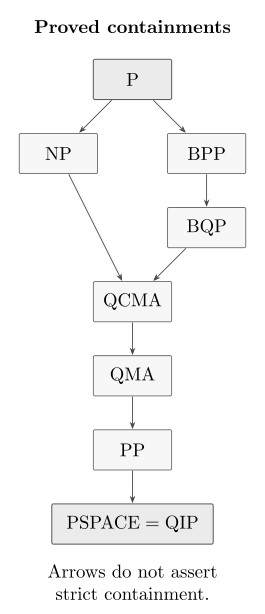
An arrow means containment, not strict containment. Its direction points toward a class that can solve at least the same problems. No arrow compares NP directly with BQP. Transitive arrows are omitted.

The upper part of the diagram follows from the simulations just described. The counting-complexity upper bounds give

$$\mathrm{BQP}\subseteq\mathrm{QMA} \subseteq\mathrm{PP}\subseteq\mathrm{PSPACE}.$$

The last inclusion can be understood by enumerating a polynomial-time probabilistic machine’s computation branches using polynomial workspace and keeping a counter of polynomial bit length. The time can be exponential. Adleman, DeMarrais and Huang established the BQP-to-PP upper bound; Watrous reviews these containments and their formulations.

It remains unknown whether BPP equals BQP, whether NP is contained in BQP, whether BQP is contained in NP, and whether QCMA equals QMA in the ordinary unrelativized setting. BQP versus PSPACE and P versus NP also remain unresolved. Drawing separate boxes does not prove a separation.

The distinction is useful in practice: an efficient quantum algorithm is a constructive upper bound, whereas proving that no efficient classical algorithm exists is a different theorem.

Oracle comparisons and what they imply

An oracle supplies a specified query operation at unit cost. For a classical Boolean function $f$, a quantum query usually means $\lvert x,b\rangle\mapsto\lvert x,b\oplus f(x)\rangle$. The underlying function is classical even when queried in superposition. A general unitary oracle supplies a broader kind of operation.

Relativized notation such as $\mathrm{BQP}^A$ means that algorithms have access to oracle $A$. Quantum and classical algorithms receive the same underlying information, but use their respective query models.

Simon’s problem separates quantum and randomized classical query requirements exponentially. Raz and Tal proved that an oracle exists for which $\mathrm{BQP}^A\not\subseteq\mathrm{PH}^A$, where PH is the polynomial hierarchy Raz and Tal (2022).

Aaronson and Kuperberg separated QMA and QCMA relative to a quantum oracle. A separation using a classical-function oracle with quantum query access was subsequently proved by Bostanci, Haferkamp, Nirkhe and Zhandry Aaronson and Kuperberg (2007), Bostanci et al. (2025). Both are oracle separations; neither settles the ordinary QMA–QCMA question.

Such results expose the power of particular forms of access and limitations of proof techniques that relativize. They do not make a difficult oracle free to implement. Query complexity and lower bounds develop these distinctions further.

The local Hamiltonian decision problem

An input describes

$$H=\sum_{j=1}^{m}H_j$$

on $n$ qubits, with polynomially many terms, each acting on at most a fixed number $k$ of qubits. Require polynomially bounded term norms and polynomial-bit descriptions of their entries. Given $a<b$ with $b-a\ge1/\operatorname{poly}(n)$, distinguish

$$\begin{aligned} \text{YES:}\quad &\lambda_{\min}(H)\le a,\\ \text{NO:}\quad &\lambda_{\min}(H)\ge b. \end{aligned}$$

The promise excludes intermediate energies. A short binary description of a coefficient alone does not bound its magnitude: $2^n$ uses only $n+1$ bits. This is why the norm condition is separate from the description length.

The general problem is QMA-complete for fixed $k\ge2$; the two-local result is due to Kempe, Kitaev and Regev. One-local Hamiltonians are efficiently solvable by grouping all terms on each qubit and diagonalizing the resulting two-dimensional operators.

Here QMA-hard means every QMA promise problem can be transformed into this problem by a classical polynomial-time reduction preserving yes and no instances. QMA-complete adds membership in QMA. These statements are about input families and required precision, not a declaration that every individual Hamiltonian is hard.

Checking a supplied low-energy state

First take $0\le H_j\le I$. Choose $j$ uniformly and perform the local two-outcome measurement $\{I-H_j,H_j\}$, accepting the first outcome. For any witness $\rho$,

$$p_{\mathrm{acc}}(\rho) =1-\frac{\operatorname{Tr}(H\rho)}m.$$

A yes-instance has some witness accepted with probability at least $1-a/m$. On a no-instance, every state has energy at least $b$, so acceptance is at most $1-b/m$. The inverse-polynomial acceptance gap $(b-a)/m$ can be amplified. The local POVM can be implemented to sufficient accuracy because $k$ is fixed and its entries are efficiently specified.

For general terms $K_j$ with a known common norm bound $J>0$, use

$$H_j=\frac{K_j+JI}{2J}.$$

This changes the energy thresholds to $(a+mJ)/(2J)$ and $(b+mJ)/(2J)$, and the acceptance gap becomes $(b-a)/(2Jm)$. Polynomial $J$ preserves an inverse-polynomial gap; exponential $J$ need not.

Worked example: noncommuting terms on one qubit

Consider

$$\begin{aligned} H_1&=\frac{I-X}{2},\qquad H_2=\frac{I-Z}{2},\\ H&=I-\frac{X+Z}{2}. \end{aligned}$$

Each term has minimum eigenvalue zero, but their minimizing states differ. The sum has energies

$$E_\pm=1\pm\frac1{\sqrt2}.$$

Its ground state’s Bloch vector is $(1,0,1)/\sqrt2$. The uniform term-sampling verifier accepts this state with probability

$$1-\frac{E_-}{2} =\frac12+\frac1{2\sqrt2} \approx0.853553.$$

The largest basis-state acceptance is only $0.75$. The example shows both why energies of incompatible local terms cannot be minimized separately and how a quantum witness improves acceptance. It remains an easy one-qubit calculation, not a hard instance.

Encoding computation in a ground-energy question

The Feynman–Kitaev construction represents a verifier computation through a history state,

$$\begin{aligned} \lvert\eta\rangle&= \frac1{\sqrt{T+1}}\sum_{t=0}^{T} \lvert t\rangle_{\mathrm{clock}}\lvert\psi_t\rangle_{\mathrm{work}},\\ \lvert\psi_t\rangle&=U_t\cdots U_1\lvert\psi_0\rangle. \end{aligned}$$

Initialization, valid-clock, propagation and final-output penalties enforce the computation. An accepting witness produces a low-energy state. The harder direction is proving that no state—not merely no proposed history state—can evade the penalties on a no-instance. That soundness argument supplies an inverse-polynomial energy separation. Local clock encodings and interaction reductions give the constant-locality completeness theorem; see Kitaev, Shen and Vyalyi and Kempe, Kitaev and Regev (2006).

Ground-state preparation, deciding an energy promise and following a supplied gapped path are different tasks. A particular integrable, commuting, stoquastic, geometrically restricted or gapped family requires its own complexity result. QMA-completeness does not imply that every variational calculation or finite-temperature observable is hard. Lattice models develops the physical families; adiabatic computation explains the separate path-following problem.

Interaction with an untrusted prover

QIP permits polynomially many polynomial-size quantum messages between an efficient quantum verifier and one computationally unbounded prover. Completeness requires an honest strategy that succeeds on yes-instances; soundness bounds every cheating strategy on no-instances. The prover can retain private quantum memory between messages.

Jain, Ji, Upadhyay and Watrous proved

$$\mathrm{QIP}=\mathrm{PSPACE}.$$

The containment in PSPACE uses semidefinite-program descriptions and matrix multiplicative weights. The reverse inclusion follows from $\mathrm{IP}=\mathrm{PSPACE}$, since classical interactive proofs are included Jain et al. (2011). This equality does not turn an unaided BQP computer into a PSPACE solver: interaction with the prover is part of the resource.

One message yields QMA; a classical message yields QCMA. Multiple separated provers, pre-shared entanglement and zero-knowledge conditions define other models and cannot be inferred from the single-prover equality. The complexity-class glossary provides a shorter lookup, including postselection.

Exercises

1. Amplify bounded error

Repeat a BQP circuit independently an odd number $k$ of times and accept by majority. Bound its error when the original completeness is $2/3$ and soundness $1/3$. Compute the exact worst-case error for $k=3$.

Solution

A majority error requires the sample frequency to deviate by at least $1/6$ from its mean. Hoeffding’s inequality gives $\Pr[\mathrm{error}]\le e^{-k/18}$ on either promised case. Thus logarithmically many repetitions in $1/\epsilon$ suffice for error $\epsilon$. At $k=3$, the no-instance worst case is $3(1/3)^2(2/3)+(1/3)^3=7/27$; the yes-instance error is the same. The general bound is sufficient, not tight for this small $k$.

2. Prove the easy containments

Explain $\mathrm{BPP}\subseteq\mathrm{BQP}\subseteq\mathrm{QCMA} \subseteq\mathrm{QMA}$, including why the last simulation is sound against coherent witnesses.

Solution

Hadamards supply random bits and reversible classical computation reproduces a BPP algorithm. A QCMA verifier can ignore its witness and run BQP. For QCMA inside QMA, measure the witness bits before running the original QCMA verifier. Acceptance is then a weighted average over classical strings, each bounded by the soundness threshold on a no-instance.

3. Find the best witness

For $Q=I/2+3X/10$, find the maximum acceptance probability, an optimal witness and the best probability when the witness is first dephased in the computational basis. Does the difference prove QCMA differs from QMA?

Solution

The eigenvalues are $4/5$ and $1/5$, with eigenvectors $\lvert+\rangle$ and $\lvert-\rangle$. The maximum is $4/5$. Dephasing sets the $X$ expectation to zero, leaving acceptance $1/2$. This distinguishes two procedures for one verifier. QCMA permits a different verifier that interprets a classical instruction and prepares $\lvert+\rangle$, so the example proves no class separation.

4. Normalize an energy verifier

For $K=\sum_{j=1}^m K_j$ with $\lVert K_j\rVert\le J$, derive the uniform term-sampling acceptance probability after shifting and rescaling. What assumption keeps a gap $b-a$ inverse polynomial in the acceptance probabilities?

Solution

Use $H_j=(K_j+JI)/(2J)$, so

$$p_{\mathrm{acc}}(\rho) =\frac12-\frac{\operatorname{Tr}(K\rho)}{2Jm}.$$

The completeness–soundness gap is $(b-a)/(2Jm)$. Polynomially many terms and polynomially bounded $J$, together with an inverse-polynomial $b-a$, preserve the needed gap. Polynomial-bit coefficient descriptions alone do not imply a polynomial norm bound.

5. Recognize the promise

For thresholds $a=0.20$, $b=0.25$, classify ground energies $0.18$, $0.23$ and $0.27$. Does the algorithm have to announce that an input is outside the promise?

Solution

The first is yes and the last no. The middle is outside the promise, where either output is permitted. The algorithm need not detect or announce the violation. Its guaranteed behavior is restricted to promised inputs.

6. Distinguish oracle and ordinary separations

An oracle $A$ satisfies $\mathrm{BQP}^A\not\subseteq\mathrm{BPP}^A$. Does replacing its queries by an explicit circuit automatically prove $\mathrm{BQP}\ne\mathrm{BPP}$?

Solution

No. The oracle theorem applies to the specified black-box access model. An explicit implementation may be expensive, and its description may expose structure unavailable to a black-box classical algorithm. Neither the oracle’s implementation nor an ordinary classical lower bound follows from the relativized separation.

7. Read containment arrows

A proposed diagram asserts $\mathrm{NP}\subseteq\mathrm{BQP}\subsetneq\mathrm{QMA}$. Which claims follow from the definitions and results above?

Solution

Only $\mathrm{BQP}\subseteq\mathrm{QMA}$ is established here. NP versus BQP and strictness of BQP inside QMA are open. The correct diagram can place NP and BQP below QCMA without drawing an arrow between NP and BQP or asserting strict containments.

References

• Scott Aaronson and Greg Kuperberg, “Quantum Versus Classical Proofs and Advice,” Theory of Computing 3(7), 129–157 (2007), doi:10.4086/toc.2007.v003a007.
• Leonard M. Adleman, Jonathan DeMarrais, and Ming-Deh A. Huang, “Quantum Computability,” SIAM Journal on Computing 26(5), 1524–1540 (1997), doi:10.1137/S0097539795293639.
• Sanjeev Arora and Boaz Barak, Computational Complexity: A Modern Approach, Cambridge University Press (2009), doi:10.1017/CBO9780511804090.
• Ethan Bernstein and Umesh Vazirani, “Quantum Complexity Theory,” SIAM Journal on Computing 26(5), 1411–1473 (1997), doi:10.1137/S0097539796300921.
• John Bostanci, Jonas Haferkamp, Chinmay Nirkhe, and Mark Zhandry, “Separating QMA from QCMA with a Classical Oracle,” arXiv:2511.09551 (2025), arXiv:2511.09551.
• Rahul Jain, Zhengfeng Ji, Sarvagya Upadhyay, and John Watrous, “QIP = PSPACE,” Journal of the ACM 58(6), article 30 (2011), doi:10.1145/2049697.2049704.
• Julia Kempe, Alexei Kitaev, and Oded Regev, “The Complexity of the Local Hamiltonian Problem,” SIAM Journal on Computing 35(5), 1070–1097 (2006), doi:10.1137/S0097539704445226.
• Alexei Yu. Kitaev, Alexander H. Shen, and Mikhail N. Vyalyi, Classical and Quantum Computation, Graduate Studies in Mathematics 47, American Mathematical Society (2002), doi:10.1090/gsm/047.
• Chris Marriott and John Watrous, “Quantum Arthur–Merlin Games,” Computational Complexity 14, 122–152 (2005), doi:10.1007/s00037-005-0194-x.
• Ran Raz and Avishay Tal, “Oracle Separation of BQP and PH,” Journal of the ACM 69(4), article 30 (2022), doi:10.1145/3530258.
• Daniel R. Simon, “On the Power of Quantum Computation,” SIAM Journal on Computing 26(5), 1474–1483 (1997), doi:10.1137/S0097539796298637.
• John Watrous, “Quantum Computational Complexity,” in Encyclopedia of Complexity and Systems Science, Springer, 7174–7201 (2009), arXiv:0804.3401.