Algorithmic Primitives

Quantum algorithms reuse a small collection of ideas: prepare a state, access a function coherently, encode information in relative phases, interfere amplitudes, amplify a desired outcome, and extract a useful result. These are algorithmic primitives. Learning how they fit together makes apparently different algorithms easier to recognize and understand.

A primitive does not by itself establish a speedup. Its input must be available, its output must suit the next step, and its cost must be included. The final result may be a classical answer or a prepared quantum state for further processing.

Helpful background. The circuit model explains registers and measurements; probability amplitudes explains interference; universal gate sets explains how abstract operations are synthesized.

State preparation and coherent access

Hadamards cheaply prepare a uniform state on $N=2^n$ basis labels:

$$H^{\otimes n}|0^n\rangle=\frac1{\sqrt N}\sum_x|x\rangle.$$

One measurement still returns only one label. More general preparation, $\mathcal A|0\rangle=\sum_x\sqrt{p_x}e^{i\theta_x}|x\rangle$, can be expensive: amplitudes stored in a classical list are not automatically available as a quantum state.

A reversible Boolean query acts as

$$O_f|x\rangle|y\rangle=|x\rangle|y\oplus f(x)\rangle.$$

With target $|0\rangle$, it correlates the registers:

$$\sum_x\alpha_x|x\rangle|0\rangle \longmapsto\sum_x\alpha_x|x\rangle|f(x)\rangle.$$

With target $|-\rangle$, it instead gives a clean phase pattern,

$$\sum_x\alpha_x|x\rangle|-\rangle \longmapsto\sum_x\alpha_x(-1)^{f(x)}|x\rangle|-\rangle.$$

The target returns to its original state. This is phase kickback, not a measurement of all function values. An actual reversible implementation may use temporary workspace, which must be restored if it would otherwise distinguish interfering paths. Quantum oracles explains when inverse, controlled or powered queries are available; those capabilities do not follow from the name of an operation alone.

Turning relative phase into probability

The simplest interference example is $H\,\operatorname{diag}(1,e^{i\phi})\,H|0\rangle$. The first Hadamard creates two alternatives, the middle gate changes their relative phase, and the final Hadamard recombines them:

$$|\psi_{\mathrm{out}}\rangle =\frac{1+e^{i\phi}}2|0\rangle +\frac{1-e^{i\phi}}2|1\rangle.$$

Therefore $P(0)=\cos^2(\phi/2)$ and $P(1)=\sin^2(\phi/2)$. Before the last Hadamard, measuring in the computational basis would give equal probabilities for every $\phi$. The useful information lies in the relative phase until the readout basis is changed.

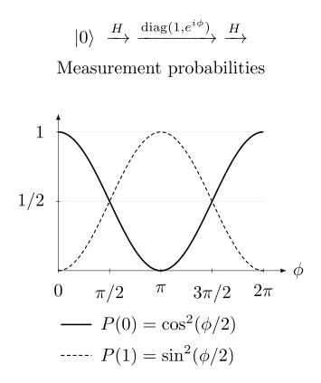
The final Hadamard converts relative phase to a measurable probability. At $\phi=\pi$, destructive interference eliminates the zero outcome and the one outcome is certain.

For many qubits, the Walsh–Hadamard transform gives

$$b_y=\frac1{\sqrt N}\sum_x(-1)^{x\cdot y}a_x, \qquad \sum_y|b_y|^2=\sum_x|a_x|^2.$$

Here the dot product is modulo two. Useful phases reinforce some outputs and cancel others while conserving total probability. Deutsch–Jozsa detects the constant-versus-balanced promise, Bernstein–Vazirani recovers a linear character, and Simon combines related interference with sampling and classical linear algebra.

Fourier transformation and phase estimation

The quantum Fourier transform maps

$$F_N|x\rangle=\frac1{\sqrt N}\sum_{k=0}^{N-1}e^{2\pi ixk/N}|k\rangle.$$

For $N=2^n$, its usual exact circuit has $O(n^2)$ gates in a gate set with the required controlled rotations; synthesis into a fixed alphabet adds precision-dependent cost. It transforms amplitudes but does not output a classical list of all Fourier coefficients. The classical FFT has a different input and output task.

Phase estimation combines this transform with controlled evolution. Let $U|u_j\rangle=e^{2\pi i\phi_j}|u_j\rangle$ and use $m$ controls, $M=2^m$. After controlled powers and inverse Fourier decoding, the control state for eigenphase $\phi$ is

$$|\eta_m(\phi)\rangle=\sum_{y=0}^{M-1}g_y(\phi)|y\rangle, \qquad g_y(\phi)=\frac1M\sum_{k=0}^{M-1}e^{2\pi ik(\phi-y/M)}.$$

If $\phi=y_0/M$, only $y=y_0$ survives. Otherwise several outcomes have nonzero amplitudes. For an input $\sum_jc_j|u_j\rangle$ in an orthonormal eigenbasis, the joint state and measured law are

$$\sum_jc_j|\eta_m(\phi_j)\rangle|u_j\rangle, \qquad P(y)=\sum_j|c_j|^2|g_y(\phi_j)|^2.$$

Finite precision does not literally return an eigenstate index: nearby phases can give overlapping outcome distributions. Even ideal phase measurement preserves coherence within a degenerate eigenspace. Overlap with the desired eigenspace controls its chance of appearing.

Controlled powers $U^{2^r}$ require $M-1$ base-$U$ uses if built by repetition. Treating each power as one query changes the access model. Phase estimation develops its precision and confidence bounds; Shor’s algorithm combines efficient modular powers with classical number-theoretic recovery.

Amplifying a selected subspace

Let $\Pi_G$ project onto useful outcomes and assume $0<a<1$. Write

$$|\psi\rangle=\mathcal A|0\rangle =\sin\theta|G\rangle+\cos\theta|B\rangle, \qquad a=\sin^2\theta.$$

The normalized vectors $|G\rangle$ and $|B\rangle$ lie in the good and bad subspaces. Define the two reflections

$$S_G=I-2\Pi_G,\qquad R_\psi=2|\psi\rangle\langle\psi|-I =\mathcal A(2|0\rangle\langle0|-I)\mathcal A^\dagger.$$

Then $Q=R_\psi S_G$ rotates their plane and gives

$$Q^r|\psi\rangle =\sin((2r+1)\theta)|G\rangle +\cos((2r+1)\theta)|B\rangle.$$

This explicitly fixes the reflection sign and execution order. The endpoints are separate: $a=1$ is already successful, while $a=0$ has no good component to amplify. For a small nonzero $a$, ordinary independent preparation needs mean $1/a$ trials; suitable coherent amplification uses $O(1/\sqrt a)$ preparation, inverse and reflection calls. It requires coherent access to all those operations. Unknown success probability needs an appropriate schedule, since too many iterations can lower success again.

Amplitude amplification explains schedules and exact variants. Grover search is its uniform-state example; amplitude estimation estimates $a$ by analyzing the rotation phases.

Hamiltonian and matrix access

In units $\hbar=1$, Hamiltonian simulation approximates $e^{-iHt}$ for a specified Hermitian matrix or a carefully defined operator problem. Access might mean local terms, sparse-matrix queries, a sum of implementable unitaries, or a block encoding. Its cost depends on that access, time and error tolerance. Producing uncontrolled evolution does not automatically provide its controlled version; a later phase-estimation algorithm needs that additional capability.

The Hamiltonian simulation algorithms page compares methods, while Hamiltonian simulation connects norm errors to physical outputs. Simulating a state is different from reconstructing its entire wavefunction; observable estimation still needs measurements.

For a general matrix $A$, an $(\alpha,a,\epsilon)$ block encoding is a unitary $U_A$ whose all-zero ancilla block $B$ obeys

$$B=(\langle0^a|\otimes I)U_A(|0^a\rangle\otimes I), \qquad \|A-\alpha B\|_{\mathrm{op}}\leq\epsilon, \quad \alpha>0.$$

In the exact case $B=A/\alpha$ and $\alpha\geq\|A\|_{\mathrm{op}}$. Applying $U_A$ and measuring zero ancillas yields $A|\psi\rangle/\alpha$ with probability $\|A|\psi\rangle\|^2/\alpha^2$. The normalized output exists only if that probability is positive.

For example, take $A=\operatorname{diag}(1,1/2)$, $\alpha=1$ and $|\psi\rangle=|+\rangle$. Success is $5/8$ and the conditional state is $(2|0\rangle+|1\rangle)/\sqrt5$. Increasing $\alpha$ to two leaves that state unchanged but reduces success to $5/32$. Preparing the input and building $U_A$ may cost more than the subsequent manipulation.

Polynomial transformations of a signal

Quantum signal processing interleaves a signal unitary with chosen phase rotations. A common one-qubit signal is

$$W(x)=\begin{pmatrix}x&i\sqrt{1-x^2}\\i\sqrt{1-x^2}&x\end{pmatrix}, \qquad -1\leq x\leq1.$$

Products of $W(x)$ and $e^{i\phi_j Z}$ produce polynomial responses with degree, parity and unitarity constraints. For instance, with two signal calls and no phases, $(W(x)^2)_{00}=2x^2-1$. This is a bounded even response, not an arbitrary degree-two function. The number of signal calls is tied to polynomial degree.

For a block encoding of $A/\alpha$, singular-value transformation acts on normalized singular values $\sigma_k/\alpha$. Odd polynomial transformations map right singular vectors to left ones; even transformations act within a right or left singular space, according to the chosen projected block. Zero singular spaces and $p(0)$ also matter. One should not replace this by a generic eigenvalue formula for a non-Hermitian matrix.

Hamiltonian evolution requires the signed eigenvalues of a Hermitian operator. Its response $e^{-itx}=\cos(tx)-i\sin(tx)$ has both even and odd parts; it is not one fixed-parity real singular-value polynomial. Appropriate signal-processing constructions combine the needed responses. See block encodings and QSVT for the exact admissibility rules, and qubitization and quantum signal processing for Hamiltonian-specific constructions.

Reciprocal approximations need a spectral interval excluding zero, and sharp filters need a resolved transition region. These restrictions determine degree and retain conditioning, gap and normalization costs. Quantum linear algebra and quantum walks show how the primitives fit complete tasks.

Measurement, postselection and total cost

A measurement outcome may have several unobserved Kraus labels:

$$\widetilde\rho_y=\sum_\mu K_{y\mu}\rho K_{y\mu}^\dagger, \qquad p_y=\operatorname{Tr}\widetilde\rho_y, \qquad \rho_y=\widetilde\rho_y/p_y\quad(p_y>0).$$

Keeping only chosen outcomes is postselection. For repeatable preparations, independent trials need mean $1/p_y$ attempts per success. Repeating an unknown consumed input requires a separate way to restore it. If the whole preparation, its inverse and a success reflection are coherently available, amplitude amplification can improve the dependence toward $1/\sqrt{p_y}$. A classical success flag alone does not supply those operations.

Aaronson’s theorem $\mathrm{PostBQP}=\mathrm{PP}$ concerns a complexity model that conditions on a nonzero-probability event without charging physical repetitions. It does not turn exponentially rare experimental outcomes into an efficient procedure. Quantum instruments explains outcome probabilities and conditional states.

When composing primitives, keep query calls, gate synthesis, preparations, measured samples and classical work distinct. Approximations must be controlled in a metric that bounds the final result. Coherent errors need not cancel, and postselection can magnify errors when acceptance is small. A benchmark should compare the same input access, output, accuracy and success probability for both methods.

Exercises

Superposition is not bulk readout

Prepare $H^{\otimes n}\lvert0^n\rangle$ and measure in the computational basis. What is the probability of observing a specified string $x_0$? How many independent shots are expected before that string appears?

Solution

Every basis state has amplitude $1/\sqrt N$, where $N=2^n$, so

$$\Pr(x_0) = \frac1N = 2^{-n}.$$

Independent repetition gives a geometric waiting time with mean

$$\mathbb E[T]=N=2^n.$$

Preparing a superposition does not make a specified label likely. A useful algorithm must use phase and interference to concentrate probability or extract a global property.

Compose with a supplied phase oracle

Assume the clean phase-oracle interface

$$P_f\lvert x\rangle = (-1)^{f(x)}\lvert x\rangle$$

is supplied. Derive its action on an arbitrary input superposition and state what further steps are needed to obtain a useful answer.

Solution

By linearity, an input superposition becomes

$$P_f\sum_x\alpha_x\lvert x\rangle = \sum_x\alpha_x(-1)^{f(x)}\lvert x\rangle.$$

The interface supplies a relative phase pattern, not a readable answer. A complete algorithm must still specify the interference step, measurement and postprocessing, success criterion, query model, and implementation costs. If the phase oracle is constructed from other operations, its preparation and workspace cleanup must also be included.

Read a linear phase pattern

Let $s,x\in\{0,1\}^n$ and prepare

$$\lvert\psi_s\rangle = \frac1{\sqrt N} \sum_x (-1)^{s\cdot x} \lvert x\rangle.$$

Show that $H^{\otimes n}\lvert\psi_s\rangle=\lvert s\rangle$.

Solution

The amplitude of output $y$ is

$$\begin{aligned} b_y &= \frac1N \sum_x (-1)^{s\cdot x} (-1)^{x\cdot y} \\ &= \frac1N \sum_x (-1)^{x\cdot(s\oplus y)}. \end{aligned}$$

If $y=s$, every term equals $1$, so $b_s=1$. If $y\neq s$, choose a bit where $s\oplus y$ is $1$; pairing strings that differ in that bit cancels the sum, so $b_y=0$. Hence the transformed state is exactly $\lvert s\rangle$.

This is a clean example of a relative-phase pattern becoming one deterministic classical label through interference.

Phase estimation on a superposition

Suppose two orthonormal eigenstates obey $U\lvert u_j\rangle=e^{2\pi i\phi_j}\lvert u_j\rangle$, with distinct, exactly representable phases, and the normalized system input is

$$c_0\lvert u_0\rangle+c_1\lvert u_1\rangle.$$

Assuming ideal phase resolution, give the state before measurement and the probabilities of the two phase outcomes.

Solution

Linearity gives

$$c_0 \lvert\phi_0\rangle \lvert u_0\rangle + c_1 \lvert\phi_1\rangle \lvert u_1\rangle.$$

If the phase-register states are distinguishable, measurement returns $\phi_0$ with probability $\lvert c_0\rvert^2$ and $\phi_1$ with probability $\lvert c_1\rvert^2$. The corresponding system register is projected onto the associated eigenstate.

Finite resolution broadens the phase distributions, and degenerate or nearby phases require a more careful measurement analysis.

Grover-scale amplification

There is one marked item among $N$ equally weighted inputs, so $a=1/N$ and $\sin\theta=1/\sqrt N$. Estimate the number of amplitude-amplification iterations that first brings the success probability near one.

Solution

After $r$ iterations, the good amplitude is

$$\sin\!\left((2r+1)\theta\right).$$

Choose

$$(2r+1)\theta \approx \frac\pi2.$$

For large $N$, $\theta\approx1/\sqrt N$, so

$$r \approx \frac\pi4\sqrt N-\frac12.$$

Thus the number of coherent oracle and reflection uses is $O(\sqrt N)$, compared with $O(N)$ classical trials in the same unstructured-query model.

Block-encoding success probability

An exact block encoding has normalization $\alpha$. For a normalized input $\lvert\psi\rangle$, derive the probability of measuring all ancillas in $\lvert0^a\rangle$. What happens if $\alpha$ is doubled while $A$ is fixed?

Solution

The all-zero ancilla component is

$$\frac{ A\lvert\psi\rangle }{\alpha}.$$

Therefore

$$p_0 = \frac{ \langle\psi\rvert A^\dagger A \lvert\psi\rangle }{\alpha^2}.$$

Doubling $\alpha$ divides the success probability by four. A block encoding with an unnecessarily large normalization can impose a major postselection or amplification cost even if each signal query is cheap.

Count rare accepted outcomes

A repeatable known-state preparation succeeds only when an ancilla outcome occurs with probability $p=2^{-n}$. The accepted branch has a polynomial-size circuit. What is the expected repetition cost, and why is the accepted circuit size alone not an efficiency proof?

Solution

Independent repetition requires

$$\frac1p=2^n$$

runs on average for one accepted event. The complete expected cost is therefore exponential even though each accepted branch has polynomial circuit size.

If a coherent preparation, inverse, and success reflection are available, amplitude amplification can reduce the scaling toward

$$\frac1{\sqrt p}=2^{n/2},$$

which is still exponential. An efficiency claim must include raw trials, coherent amplification resources if used, and the probability of every heralding condition.

References

• S. Aaronson, “Quantum computing, postselection, and probabilistic polynomial-time,” Proceedings of the Royal Society A 461, 3473–3482, 2005, doi:10.1098/rspa.2005.1546.
• G. Brassard, P. Høyer, M. Mosca, and A. Tapp, “Quantum amplitude amplification and estimation,” Contemporary Mathematics 305, 53–74, 2002, arXiv:quant-ph/0005055.
• A. Gilyén, Y. Su, G. H. Low, and N. Wiebe, “Quantum singular value transformation and beyond,” in Proceedings of the 51st Annual ACM SIGACT Symposium on Theory of Computing, 193–204, 2019, doi:10.1145/3313276.3316366.
• G. H. Low and I. L. Chuang, “Optimal Hamiltonian simulation by quantum signal processing,” Physical Review Letters 118, 010501, 2017, doi:10.1103/PhysRevLett.118.010501.
• M. A. Nielsen and I. L. Chuang, Quantum Computation and Quantum Information, 10th anniversary ed., Cambridge University Press, 2010, doi:10.1017/CBO9780511976667.