Amplitude Estimation

Amplitude estimation turns the success probability of a reversible quantum preparation into a classical numerical estimate. It uses the fact that amplitude amplification rotates through an angle determined by that probability: estimating the rotation angle therefore estimates the probability.

For additive error $\epsilon$ at fixed confidence, the standard coherent algorithm uses $O(1/\epsilon)$ applications of its basic iterate. Direct independent sampling uses $O(1/\epsilon^2)$ preparations. The coherent algorithm needs stronger access—including an inverse preparation and controlled operations—and a query reduction does not by itself imply the same reduction in gates or runtime.

Helpful background. Amplitude amplification develops the two-reflection rotation. Quantum phase estimation explains controlled powers and Fourier decoding. Quantum oracles distinguishes those operations from ordinary oracle access.

The probability to be estimated

Work in a finite-dimensional Hilbert space with a normalized reference state $|0\rangle$. A measurement-free unitary $\mathcal A$ and an orthogonal projector $\Pi_G$ define

$$|\psi\rangle=\mathcal A|0\rangle, \qquad a=\langle\psi|\Pi_G|\psi\rangle\in[0,1].$$

For $0<a<1$, normalize the two projected components:

$$|G\rangle = \frac{\Pi_G|\psi\rangle}{\sqrt a}, \qquad |B\rangle = \frac{(I-\Pi_G)|\psi\rangle}{\sqrt{1-a}}.$$

They are orthonormal because $\Pi_G(I-\Pi_G)=0$, and the prepared state is

$$|\psi\rangle = \sqrt a\,|G\rangle + \sqrt{1-a}\,|B\rangle = \sin\theta\,|G\rangle + \cos\theta\,|B\rangle,$$

where

$$\theta=\arcsin\sqrt a\in(0,\pi/2).$$

The endpoint cases must be handled without dividing by a vanishing norm. If $a=0$, the prepared state is entirely bad. If $a=1$, it is entirely good. Both cases have well-defined phase-estimation behavior, derived below, even though one of the normalized vectors is unnecessary.

For requested $\epsilon>0$ and $0<\delta<1$, the output is a classical random variable $\widetilde a\in[0,1]$ with a statement of the form

$$\Pr\!\left(|\widetilde a-a|\le\epsilon\right)\ge1-\delta.$$

This is an estimation task, not a search task. It does not return a good witness, expose every basis amplitude, or leave $a$ encoded as a reusable exact quantum number. Additive and relative error are different accuracy requirements, and a one-run constant-confidence theorem is different from a protocol whose failure probability is chosen by the user.

Preparation, reflections and controlled operations

The standard construction starts from four coherent components:

$$\mathcal A, \qquad \mathcal A^\dagger, \qquad S_G=I-2\Pi_G, \qquad S_0=I-2|0\rangle\langle0|.$$

Their ordered product defines the exact amplitude-amplification iterate

$$Q=-\mathcal A S_0\mathcal A^\dagger S_G.$$

The leading minus sign fixes a unitary representative, not merely a ray. It is irrelevant when a fixed number of uncontrolled iterates is followed by a measurement, because it then produces only an overall phase. It becomes a relative phase when $Q$ is applied conditionally, so standard amplitude estimation must preserve it.

The primary phase-estimation implementation chooses $M=2^m$ with $m\ge1$ and requires controlled $Q^{2^j}$ for $j=0,\ldots,m-1$. These are separate capabilities:

• a known gate circuit can be compiled into a controlled circuit, with its phases tracked and an additional implementation cost; an unknown oracle does not automatically provide controlled access;
• controlled $Q$ does not automatically make $Q^{2^j}$ a unit-cost primitive;
• a native powered oracle and $2^j$ repetitions of a base iterate have different query and depth costs;
• a measurement-based sampler does not automatically provide $\mathcal A^\dagger$ or coherent workspace cleanup.

If a controlled reflection about $|\psi\rangle$ is compiled as

$$\mathcal A\,\mathrm C(S_0)\,\mathcal A^\dagger,$$

the unconditional outer pair cancels on the control-zero branch, while the controlled reference reflection acts on the control-one branch. A controlled $S_G$ and the controlled phase associated with the leading minus sign remain necessary. Other valid compilations may distribute controls differently, but their component costs must be stated rather than hidden inside the symbol $\mathrm C(Q)$.

The circuit also uses an $m$-qubit phase register, an inverse Quantum Fourier Transform, one control-register measurement, and classical evaluation of $\sin^2(\pi Y/M)$. Approximate reflections, arithmetic, synthesized rotations, garbage registers, and measurement noise contribute additional errors.

The two Grover eigenphases

Conjugating the reference reflection gives

$$\mathcal A S_0\mathcal A^\dagger = I-2|\psi\rangle\langle\psi|.$$

In the ordered basis $\{|G\rangle,|B\rangle\}$, multiplication by $S_G$ and the leading minus sign yields

$$Q = \begin{pmatrix} 1-2a & 2\sqrt{a(1-a)}\\ -2\sqrt{a(1-a)} & 1-2a \end{pmatrix} = \begin{pmatrix} \cos2\theta & \sin2\theta\\ -\sin2\theta & \cos2\theta \end{pmatrix}.$$

Thus $Q$ is a rotation through $-2\theta$ in real coordinate convention. Its complex eigenvectors are

$$|\psi_\pm\rangle = \frac{|G\rangle\pm i|B\rangle}{\sqrt2},$$

and direct multiplication gives

$$Q|\psi_\pm\rangle = e^{\pm2i\theta}|\psi_\pm\rangle.$$

The prepared state has equal squared overlap with the two eigenvectors:

$$|\psi\rangle = \frac{-i}{\sqrt2} \left( e^{i\theta}|\psi_+\rangle - e^{-i\theta}|\psi_-\rangle \right).$$

Writing an eigenvalue as $e^{2\pi i\phi}$ therefore produces the conjugate phases

$$\phi_+=\frac{\theta}{\pi}, \qquad \phi_-=1-\frac{\theta}{\pi}\pmod1.$$

These phases encode the same probability because $\sin^2(\pi\phi_+)=\sin^2(\pi\phi_-)=a$. Replacing $Q$ by $-Q$ instead shifts both phases by $1/2$. For even $M$, the output distribution is translated by $M/2$ modulo $M$, and the decoded random estimate is complemented: $\widetilde a\mapsto1-\widetilde a$. On an exact-grid instance, the wrong representative therefore returns exactly $1-a$.

From a phase register to a probability estimate

Take $M=2^m$ with $m\ge1$. Prepare the control register uniformly and the work register as $|\psi\rangle$:

$$\frac1{\sqrt M} \sum_{j=0}^{M-1}|j\rangle|\psi\rangle.$$

The controlled-power stage implements $|j\rangle|\xi\rangle\mapsto|j\rangle Q^j|\xi\rangle$. Substituting the eigenvector decomposition gives

$$\frac{-i}{\sqrt{2M}} \sum_{j=0}^{M-1}|j\rangle \left( e^{i(2j+1)\theta}|\psi_+\rangle - e^{-i(2j+1)\theta}|\psi_-\rangle \right).$$

Each orthogonal work-register branch carries the ordinary phase gradient for $\phi_+$ or $\phi_-$. Apply the inverse Fourier transform to the control register and measure

$$Y\in\{0,1,\ldots,M-1\}.$$

The amplitude-specific classical decoder is

$$\widetilde a = \sin^2\!\left(\frac{\pi Y}{M}\right).$$

Exact outcome probabilities and phase folding

For a single eigenphase $\phi$, define the finite Fourier kernel

$$\begin{aligned} D_M(y;\phi) &= \frac1{M^2} \left| \sum_{j=0}^{M-1}e^{2\pi i j(\phi-y/M)} \right|^2 \\ &= \frac{ \sin^2\!\big(\pi M(\phi-y/M)\big) }{ M^2\sin^2\!\big(\pi(\phi-y/M)\big) }. \end{aligned}$$

When numerator and denominator vanish together, the value is the limiting value one. Unitarity of the inverse Fourier transform gives $\sum_yD_M(y;\phi)=1$.

The kernel follows directly from a finite geometric series. Its numerator measures the failure of the phase gradient to close after $M$ terms, while its denominator measures the separation between the true phase and the candidate grid point. This interpretation is useful but does not turn the distribution into a continuous density: $Y$ remains a discrete outcome, and the removable singularity must be assigned before numerical evaluation.

The two work-register eigenvectors are orthogonal. Tracing out that register therefore removes cross terms rather than adding amplitudes from the two branches. The exact measured law is

$$\Pr(Y=y) = \frac12 \left[ D_M\!\left(y;\frac\theta\pi\right) + D_M\!\left(y;1-\frac\theta\pi\right) \right].$$

The identities

$$D_M(y;1-\phi)=D_M(M-y;\phi)$$

and

$$\sin^2\!\left(\pi\frac{M-y}{M}\right) = \sin^2\!\left(\pi\frac yM\right)$$

show both the mirror symmetry of the distribution and why one decoder handles the two phases. Indices in the first identity are taken modulo $M$.

The factors $1/2$ are quantum overlap weights, not an extra classical coin inserted by the algorithm. A hypothetical preparation of one Grover eigenvector would give one kernel, but $\mathcal A|0\rangle$ has equal support on both. Conversely, adding the two kernel amplitudes before squaring would be wrong because their work-register labels are orthogonal.

If $M\phi$ is an integer, the corresponding branch occupies one exact bin. Off the grid, the Dirichlet-shaped kernel spreads over all bins. The nonlinear decoder then generally has finite-$M$ bias; no theorem below says that $\mathbb E[\widetilde a]=a$. The exact law, not an asymptotic normal approximation, is the appropriate object for checking small instances.

Accuracy, confidence and the endpoints

The amplitude-estimation theorem of Brassard, Høyer, Mosca, and Tapp states that, for every positive integer $k$,

$$|\widetilde a-a| \le \frac{2\pi k\sqrt{a(1-a)}}{M} + \frac{\pi^2k^2}{M^2}$$

with probability at least $8/\pi^2$ for $k=1$, and with probability strictly greater than

$$1-\frac1{2(k-1)}$$

for integer $k\ge2$. Here $k$ enlarges the accepted phase window in one run; it is not a repetition count.

To connect phase and probability carefully, fold the measured phase into $[0,\pi/2]$:

$$\widetilde\theta = \pi\min\!\left\{\frac YM,1-\frac YM\right\}.$$

Then $\widetilde a=\sin^2\widetilde\theta$. On the circular phase-window event associated with either conjugate branch, $|\widetilde\theta-\theta|\le\Delta$. Taylor’s theorem applied to $f(x)=\sin^2x$, with $f'(\theta)=\sin2\theta$ and $|f''(x)|\le2$, gives

$$\begin{aligned} |\widetilde a-a| &\le |\sin2\theta|\,\Delta+\Delta^2 \\ &= 2\sqrt{a(1-a)}\,\Delta+\Delta^2. \end{aligned}$$

Taking $\Delta=\pi k/M$ produces the stated bound. Since $\sqrt{a(1-a)}\le1/2$, the uniform one-run error is at most $\pi/M+\pi^2/M^2$ for $k=1$, which establishes the fixed-confidence scale $M=\Theta(1/\epsilon)$.

The endpoints are exact only under their stated grid conditions. At $a=0$, $Q$ has phase zero on the prepared state, so $Y=0$ and $\widetilde a=0$ with certainty. At $a=1$, the phase is $1/2$; the decoder returns one with certainty when $M$ is even, including every primary power-of-two construction with $m\ge1$. For odd $M$, phase $1/2$ lies between bins and the endpoint is not exact.

To reach a chosen confidence, repeat an odd number $R$ of independent runs that each meet the same error target and return their median. With $p_0=8/\pi^2$,

$$\Pr(\text{median fails}) \le \exp\!\left[-2R\left(p_0-\frac12\right)^2\right].$$

Thus this elementary construction uses $O((1/\epsilon)\log(1/\delta))$ base iterates. It is rigorous, but it is not a claim that this confidence dependence is optimal among all variants.

Two finite examples

Exactly representable phases

Take

$$\theta=\frac\pi8, \qquad a=\sin^2\frac\pi8=\frac{2-\sqrt2}{4}, \qquad M=8.$$

The iterate is

$$Q = \frac1{\sqrt2} \begin{pmatrix} 1&1\\ -1&1 \end{pmatrix}.$$

Its phases $1/8$ and $7/8$ are exactly on the grid, so

$y$	$\Pr(Y=y)$	$\widetilde a$
$1$	$1/2$	$(2-\sqrt2)/4$
$7$	$1/2$	$(2-\sqrt2)/4$

If the controlled circuit implements $-Q$, the phases become $5/8$ and $3/8$. The exact outcomes $5$ and $3$ decode to

$$\sin^2\frac{5\pi}{8} = \sin^2\frac{3\pi}{8} = \frac{2+\sqrt2}{4} = 1-a.$$

Three controlled-power blocks $Q,Q^2,Q^4$ contain seven repeated base iterates. This exact example isolates the sign convention: a wrong controlled sign changes the answer even with perfect gates.

Four bins and a biased estimate

Now take

$$\theta=\frac\pi6, \qquad a=\frac14, \qquad M=4.$$

Substitution into the two-kernel law gives

$y$	$\Pr(Y=y)$	$\widetilde a$
$0$	$3/16$	$0$
$1$	$3/8$	$1/2$
$2$	$1/16$	$1$
$3$	$3/8$	$1/2$

The probabilities sum to one, but the decoded mean is

$$\mathbb E[\widetilde a] = \frac38\frac12 + \frac1{16} + \frac38\frac12 = \frac7{16} \ne \frac14.$$

The decoded-error event $Y\in\{0,1,3\}$ has probability $15/16$, and every outcome in it obeys $|\widetilde a-a|\le1/4$. This directly computed event uses a tighter radius for this particular example than the general theorem supplies.

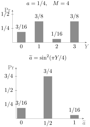
For $a=1/4$ and $M=4$, outcomes $Y=1$ and $Y=3$ both report $\widetilde a=1/2$, so their probabilities add. The lower distribution has mean $7/16$, although the true value is $1/4$. Finite bias and a probabilistic error guarantee can coexist.

Accumulated implementation error

Assume all circuit approximations in this paragraph remain unitary. Suppose the initial prepared state has vector-norm error at most $\eta_A$, every implemented controlled base iterate has operator-norm error at most $\eta_Q$, and the implemented inverse-QFT unitary has operator-norm error at most $\eta_F$. If $T=M-1$ iterates are used, telescoping and contractivity give the conservative premeasurement bound

$$\eta_A+T\eta_Q+\eta_F.$$

For normalized pure states, a vector-distance bound $\eta$ also bounds the total variation distance between their measurement distributions. Thus an ideal event with probability at least $p_0$ still has probability at least $p_0-\eta$. Choose $\eta<p_0-1/2$ before applying the median argument to the implemented circuit. Measurement noise requires an additional channel or outcome-distribution bound. The bound is a worst-case coherent budget, not a stochastic-noise model, and keeping it constant as $M$ grows requires the per-iterate error to decrease with $M$.

Query counts and direct sampling

For a matched direct-sampling baseline, prepare and measure independent Bernoulli variables $X_i\in\{0,1\}$ with $\mathbb E X_i=a$. Hoeffding’s inequality gives

$$\Pr\!\left(|\overline X_n-a|\ge\epsilon\right) \le 2e^{-2n\epsilon^2},$$

so it is sufficient to take

$$n \ge \frac{\log(2/\delta)}{2\epsilon^2}.$$

This is a theorem about independent samples from the specified Bernoulli experiment. It is not a lower bound on every classical algorithm for a structured application. The coherent comparison grants stronger access and must charge for that access.

For the primary $M=2^m$ repeated-base construction, the exact component counts are:

Resource	Count in one run
phase-register qubits	$m=\log_2M$
controlled-power blocks	$m$
repeated base $Q$ applications	$1+2+\cdots+2^{m-1}=M-1$
longest coherent power	$Q^{M/2}$
forward $\mathcal A$	$M$
inverse $\mathcal A^\dagger$	$M-1$
good reflection $S_G$	$M-1$
reference reflection $S_0$	$M-1$
inverse Fourier transforms	$1$
measurements and decoders	$1$ each

The forward count includes the initial preparation. The remaining $M-1$ forward calls and all inverse/reflection calls arise from the repeated iterate decompositions. If $Q^{2^j}$ is instead a primitive, report $m$ powered queries and the physical cost of those powers; the $M-1$ count describes a different implementation using repeated base operations.

Total query count and maximum coherent depth answer different questions. The standard controlled-power stage preserves one coherent phase register through the longest $Q^{M/2}$ block, so the repeated-base realization has sequential oracle depth of order $M$ even though it contains only $m$ labeled power blocks. Shot-based variants may distribute some circuits across independent runs, but then pay in total calls and classical inference.

At fixed nontrivial success probability, Nayak and Wu’s Boolean-mean lower bound makes the worst-case $\Theta(1/\epsilon)$ quantum-query dependence optimal for families large enough to support the requested precision, for example $N=\Omega(1/\epsilon)$. A fixed finite $N$ saturates rather than supporting an arbitrarily small-$\epsilon$ asymptotic. This lower bound belongs to the Boolean-query regime, not to every encoding of a real-world expectation.

Query counts still omit two-qubit gates, ancillas, coherent depth, arithmetic, rotation synthesis, loading, uncomputation, repetitions, inference, routing, error correction, and physical spacetime. Those quantities decide whether the query advantage survives as an end-to-end advantage.

Methods without a Fourier transform

Several alternatives measure success after selected uncontrolled powers:

$$p_r(a)=\sin^2((2r+1)\arcsin\sqrt a).$$

The inverse preparation is still needed inside $Q$. Different powers reveal different oscillations, so one must resolve their ambiguity; a single high power usually does not identify $a$.

Method	Data and guarantee
Maximum likelihood	Fit good/bad shots from a chosen set of powers. Suzuki and collaborators give asymptotic Fisher-information analysis and simulations; these alone are not finite-sample correctness bounds.
Iterative estimation	Choose powers adaptively and propagate confidence intervals. Grinko and collaborators prove finite additive-error guarantees for their specified interval construction and shot budgets.
Grover-only estimation	Aaronson and Rall give a rigorous adaptive counting method and amplitude-estimation extension without a QFT. Their relative-error and access assumptions specify the comparison.
Limited-depth estimation	Giurgica-Tiron and collaborators trade total calls against maximum sequential depth. Their power-law result assumes statistical regularity; the separate QoPrime family has a fully rigorous discrete-parameter construction.

For example, the Chernoff–Hoeffding version of Grinko and collaborators’ Theorem 1 gives an interval of width at most $2\epsilon$, containing $a$ with probability at least $1-\alpha$. With the theorem’s shot-budget conditions, its number of $Q$ applications satisfies

$$N_{\rm oracle}<\frac{50}{\epsilon} \log\!\left[\frac2\alpha\log_2\!\left(\frac\pi{4\epsilon}\right)\right]$$

in the small-error regime. This bound concerns that algorithm and interval construction, not arbitrary adaptive fits. A Fisher-information lower bound on variance does not establish an upper bound on estimation error. Noise-model studies, such as Tanaka and collaborators’, likewise apply to the specified model.

Encoding expectation values and counts

A bounded expectation becomes an amplitude only through a reversible encoder. For a distribution $p_x$ and a real function $f(x)\in[0,1]$, a coherent preparation can have the form

$$\mathcal A|0\rangle = \sum_x\sqrt{p_x}\,|x\rangle \left( \sqrt{1-f(x)}\,|0\rangle + \sqrt{f(x)}\,|1\rangle \right),$$

with any work registers coherently cleaned or explicitly retained. Declaring the flag-one subspace good gives

$$a = \sum_xp_xf(x) = \mathbb E[f(X)].$$

For $f\in[L,U]$ with $L<U$, encode

$$g(x)=\frac{f(x)-L}{U-L}\in[0,1]$$

and multiply the final additive error by $U-L$. If $L=U$, the expectation is already known. This rescaling covers signed real functions. Complex functions or non-diagonal observables need an additional explicit reduction, such as separate real and imaginary tests; the word “expectation” alone supplies no circuit.

The circuit cost includes state preparation for $p_x$, reversible evaluation of $f$, finite-precision arithmetic, the controlled rotation, garbage cleanup, and every induced bias. An efficiently indexed classical table does not automatically have an efficient coherent loader and inverse. Montanaro’s quantum Monte Carlo results give rigorous query improvements under their access assumptions, whereas Herbert exhibits a state-preparation setting in which loading costs remove the advertised speedup. These are compatible statements because they analyze different complete interfaces.

Approximate counting is the specialization in which $f$ marks $t$ of $N$ uniform inputs. Then $a=t/N$ and $\widetilde t=N\widetilde a$ satisfies, at constant confidence,

$$|\widetilde t-t| \le \frac{2\pi\sqrt{t(N-t)}}{M} + \frac{\pi^2N}{M^2}.$$

For $t>0$, a relative-error scale

$$O\!\left( \frac1{\epsilon_{\rm rel}}\sqrt{\frac Nt} \right)$$

requires a rough scale or an adaptive counting protocol; an algorithm cannot insert the unknown $t$ into its own stopping rule. Grover Search finds a marked item, whereas amplitude estimation estimates the marked fraction.

Fixed-point amplification solves a different task: it produces high success uniformly over a promised range. It does not return a numerical estimate of $a$, nor does its completed-sequence guarantee imply monotonic behavior at every intermediate step.

Exercises

1. Derive the eigenphases and folded decoder

Starting from the matrix for $Q$, derive its two normalized eigenvectors, decompose $|\psi\rangle$ into them, identify the phases $\theta/\pi$ and $1-\theta/\pi$, and prove that one $\sin^2$ decoder handles both branches.

Solution

For $c=\cos2\theta$ and $s=\sin2\theta$,

$$\begin{pmatrix}c&s\\-s&c\end{pmatrix} \begin{pmatrix}1\\ \pm i\end{pmatrix} = e^{\pm2i\theta} \begin{pmatrix}1\\ \pm i\end{pmatrix}.$$

Normalization gives $|\psi_\pm\rangle=(|G\rangle\pm i|B\rangle)/\sqrt2$. Solving for the real basis vectors and inserting $|\psi\rangle=\sin\theta|G\rangle+\cos\theta|B\rangle$ gives

$$|\psi\rangle = \frac{-i}{\sqrt2} \left(e^{i\theta}|\psi_+\rangle-e^{-i\theta}|\psi_-\rangle\right).$$

Thus each eigenbranch has weight $1/2$, with phases $\phi_+=\theta/\pi$ and $\phi_-=1-\theta/\pi$ modulo one. If outcomes near the branches are $y$ and $M-y$, then

$$\sin^2\!\left(\frac{\pi(M-y)}M\right) = \sin^2\!\left(\frac{\pi y}M\right),$$

so the decoder is branch-independent.

2. Derive the exact two-kernel law and endpoints

Derive the mixture distribution, prove mirror symmetry, and analyze $a=0$ and $a=1$ for even and odd $M$.

Solution

Conditioned on an eigenphase $\phi$, inverse-Fourier measurement has law $D_M(y;\phi)$. The work-register eigenstates are orthogonal, so tracing them out yields

$$\Pr(Y=y) = \frac12\left[D_M(y;\theta/\pi)+D_M(y;1-\theta/\pi)\right].$$

Replacing $y$ by $M-y$ interchanges the two kernels, proving mirror symmetry with indices modulo $M$. At $a=0$, the prepared state has eigenphase zero and the only outcome is $Y=0$, so the estimate is zero. At $a=1$, the phase is $1/2$. If $M$ is even, the exact bin is $M/2$ and the decoder returns one. If $M$ is odd, $M/2$ is not an integer; the finite kernel spreads over bins and the estimate is not deterministically one. The equal-mixture formula itself was derived for $0<a<1$; the endpoints follow directly from their one-dimensional prepared subspaces.

3. Reproduce the exact-grid sign calculation

For $M=8$ and $\theta=\pi/8$, reproduce both correct outcomes and show why omitting the controlled leading minus sign returns $1-a$.

Solution

The two phases are $1/8$ and $7/8$, both grid points. QPE therefore returns $1$ or $7$ with branch weights $1/2$. In either case,

$$\widetilde a = \sin^2\frac\pi8 = \frac{2-\sqrt2}{4}.$$

Using $-Q$ shifts each phase by $1/2$. Hence the bins become $1+4=5$ and $7+4=3\pmod8$. They decode as

$$\sin^2\frac{5\pi}{8} = \sin^2\frac{3\pi}{8} = \cos^2\frac\pi8 = 1-a.$$

The failure is deterministic here because every phase is exactly representable. Three power blocks $Q,Q^2,Q^4$ contain seven base iterates and have longest coherent power $Q^4$.

4. Reproduce the four-bin distribution and its bias

For $a=1/4$ and $M=4$, verify the complete distribution, expectation, decoded-error event, and operation counts.

Solution

Here $\theta/\pi=1/6$. Substitution in the two Dirichlet kernels gives

$$(p_0,p_1,p_2,p_3) = \left(\frac3{16},\frac38,\frac1{16},\frac38\right).$$

The decoder gives $(0,1/2,1,1/2)$, so

$$\mathbb E[\widetilde a] = \frac38\frac12+\frac1{16}+\frac38\frac12 = \frac7{16}.$$

Outcomes $0,1,3$ each lie within $1/4$ of $a=1/4$, and their total probability is $3/16+3/8+3/8=15/16$. The powers $Q$ and $Q^2$ use three base iterates, so the complete counts are four forward preparations; three inverse preparations; three calls to each reflection; longest power $Q^2$; and one inverse transform, two-bit measurement, and decoder.

5. Derive the operation counts and an error bound

For $M=2^m$, derive every repeated-base component count and then prove the conservative coherent implementation-error bound.

Solution

The controlled powers have exponents $1,2,\ldots,2^{m-1}$, so their sum is

$$\sum_{j=0}^{m-1}2^j=M-1,$$

and the largest block is $Q^{M/2}$. Each base $Q$ contains one forward preparation, one inverse, and both reflections. Adding the initial preparation gives $M$ forward calls and $M-1$ of each other component.

Let the initial state error be at most $\eta_A$ in vector norm. Replace ideal controlled iterates one at a time; unitarity and the operator-norm bound $\eta_Q$ make each replacement contribute at most $\eta_Q$. Replacing the inverse QFT contributes at most $\eta_F$. The triangle inequality gives

$$\left\|\,|\widetilde\Psi\rangle-|\Psi\rangle\,\right\| \le \eta_A+(M-1)\eta_Q+\eta_F.$$

This is premeasurement coherent error. A noisy measurement needs a compatible channel or outcome-distribution metric rather than an unnamed term added to the vector norm.

6. Derive precision, confidence, and the matched baseline

Derive the probability-error inequality, its worst-case query scale, the median confidence boost, and the direct-sampling Hoeffding comparator.

Solution

For $h=\widetilde\theta-\theta$, Taylor’s theorem and $|d^2(\sin^2x)/dx^2|\le2$ give

$$|\sin^2(\theta+h)-\sin^2\theta| \le 2\sqrt{a(1-a)}|h|+h^2.$$

The $k=1$ phase event has $|h|\le\pi/M$ with probability at least $p_0=8/\pi^2$. Since $\sqrt{a(1-a)}\le1/2$, choosing $M=\Theta(1/\epsilon)$ gives uniform additive error $\epsilon$ at this fixed confidence. For odd $R$ independent runs, Hoeffding applied to their success indicators yields

$$\Pr(\text{median fails}) \le e^{-2R(p_0-1/2)^2},$$

so $R=O(\log(1/\delta))$ suffices. Direct Bernoulli sampling instead obeys $\Pr(|\bar X-a|\ge\epsilon)\le2e^{-2n\epsilon^2}$, requiring $n\ge\log(2/\delta)/(2\epsilon^2)$. The comparison concerns matched access to the same encoded quantity; it is not yet a total-runtime theorem.

7. Why one power is not enough

Suppose every shot applies exactly one ordinary Grover iterate before the good/bad measurement. Compare the complete measurement distributions for $a=0$ and $a=3/4$. Can arbitrarily many such shots distinguish them? What additional power would resolve this example?

Solution

The one-iterate success probability is $p_1(a)=a(3-4a)^2$. It vanishes for both $a=0$ and $a=3/4$, so both experiments always report failure. No number of independent shots at this single power distinguishes the two probabilities. Shots at $r=0$ have success probability $p_0(a)=a$, and therefore distinguish this pair with sufficiently many samples. Combining suitable powers, or restricting the possible angle to a known interval, prevents such ambiguities in an estimation procedure.

8. Encode a signed expectation and allocate error

Let $p=(1/2,1/3,1/6)$ and $f=(-2,1,4)$. Rescale to $g=(f+2)/6$, write a normalized address–flag state, and recover $\mathbb E[f]$ from the flag-one probability. If each encoded value of $g$ has error at most $0.002$ and remains in $[0,1]$, what amplitude-estimation error suffices for total expectation error at most $0.06$? Assume the address probabilities are exact.

Solution

The rescaled values are $g=(0,1/2,1)$, giving

$$|\psi\rangle= \frac1{\sqrt2}|0\rangle|0\rangle +\frac1{\sqrt6}|1\rangle(|0\rangle+|1\rangle) +\frac1{\sqrt6}|2\rangle|1\rangle.$$

The squared amplitudes sum to $1/2+1/6+1/6+1/6=1$. The flag-one probability is $a=1/3$, and $\mathbb E[f]=6a-2=0$, agreeing with the direct weighted sum.

Encoding errors change $a$ by at most $\sum_xp_x(0.002)=0.002$. If amplitude estimation has additive error at most $0.008$ relative to the encoded probability, then

$$|\widetilde\mu-\mu|\le6(0.002+0.008)=0.06$$

on the algorithm’s stated success event. Encoding bias is systematic; taking more shots does not remove it. Other preparation, arithmetic or circuit errors would need part of the same accuracy allowance.

References

• S. Aaronson and P. Rall, “Quantum Approximate Counting, Simplified,” Proceedings of the 3rd Symposium on Simplicity in Algorithms, 24–32 (2020), doi:10.1137/1.9781611976014.5.
• G. Brassard, P. Høyer, M. Mosca, and A. Tapp, “Quantum Amplitude Amplification and Estimation,” Contemporary Mathematics 305, 53–74 (2002), doi:10.1090/conm/305/05215.
• T. Giurgica-Tiron, I. Kerenidis, F. Labib, A. Prakash, and W. Zeng, “Low Depth Algorithms for Quantum Amplitude Estimation,” Quantum 6, 745 (2022), doi:10.22331/q-2022-06-27-745.
• D. Grinko, J. Gacon, C. Zoufal, and S. Woerner, “Iterative Quantum Amplitude Estimation,” npj Quantum Information 7, 52 (2021), doi:10.1038/s41534-021-00379-1.
• S. Herbert, “No Quantum Speedup with Grover–Rudolph State Preparation for Quantum Monte Carlo Integration,” Physical Review E 103, 063302 (2021), doi:10.1103/PhysRevE.103.063302.
• W. Hoeffding, “Probability Inequalities for Sums of Bounded Random Variables,” Journal of the American Statistical Association 58, 13–30 (1963), doi:10.1080/01621459.1963.10500830.
• A. Montanaro, “Quantum Speedup of Monte Carlo Methods,” Proceedings of the Royal Society A 471, 20150301 (2015), doi:10.1098/rspa.2015.0301.
• A. Nayak and F. Wu, “The Quantum Query Complexity of Approximating the Median and Related Statistics,” in Proceedings of the 31st Annual ACM Symposium on Theory of Computing, 384–393 (1999), doi:10.1145/301250.301349.
• Y. Suzuki, S. Uno, R. Raymond, T. Tanaka, T. Onodera, and N. Yamamoto, “Amplitude Estimation without Phase Estimation,” Quantum Information Processing 19, 75 (2020), doi:10.1007/s11128-019-2565-2.
• T. Tanaka, Y. Suzuki, S. Uno, R. Raymond, T. Onodera, and N. Yamamoto, “Amplitude Estimation via Maximum Likelihood on Noisy Quantum Computer,” Quantum Information Processing 20, 293 (2021), doi:10.1007/s11128-021-03215-9.