Quantum Machine Learning

Quantum machine learning uses quantum states, circuits or measurements to learn from examples. A circuit can estimate a similarity between inputs, produce a classification score, generate samples, or process quantum systems whose information has not yet been reduced to classical measurement records. These are different learning problems. Their usefulness depends on what the input contains, how it is supplied, which prediction is needed and how well the learned model performs on new examples.

This page develops kernels, variational classifiers and Born models through small calculations. It separates three questions: can the model represent a useful predictor, can training find it, and does it generalize? Conditional quantum speedups and classical simulation results address particular tasks; neither settles all three questions for an arbitrary dataset.

Helpful background. Algorithmic primitives explains coherent input access and measurement outputs; variational algorithms introduces parameterized circuits and gradients; and random variables supplies expectations and independent sampling.

Quantum learning and the predicted quantity

Let $(X,Y)$ have a distribution $\mathcal D$. A supervised learner uses examples $(x_i,y_i)$ to choose a predictor $h$ from a family $\mathcal H$. A loss $\ell(h(x),y)$ specifies what counts as a good prediction. A class label, a real-valued score and an estimated class probability are different outputs: the same circuit can support each, but the decision rule and loss change.

Other tasks have other outputs. A generative model may supply samples without efficiently evaluating their probabilities. A quantum-state learner may predict a few observables without reconstructing a density matrix. Producing a quantum state does not automatically give a classical list of its amplitudes. This distinction matters because reading a long output can remove a saving in an intermediate calculation. Biamonte and collaborators survey the main model families Biamonte et al. (2017).

For ordinary prediction, training examples determine the fitted parameters; validation examples help choose such features as the encoding or regularization; fresh test examples estimate the selected model’s performance. Using test outcomes to tune the model makes those outcomes part of training or selection. Independent testing is then needed again. Measurement shots estimate a circuit expectation; new labeled examples estimate performance across a population. More shots on the same examples do not replace more examples.

Classical features and quantum input access

The word data can refer to resources that support very different operations.

Input supplied	What the learner can do	What still takes work
Explicit classical array	Read, copy and preprocess entries	Reading the array and preparing its quantum encoding
Classical samples	Draw examples from a distribution	Obtaining enough examples; arbitrary entry queries need additional access
Reversible value oracle	Query values coherently, such as $O_x\lvert j,b\rangle=\lvert j,b\oplus x_j\rangle$	Constructing the memory or circuit, finite precision and each invocation
Amplitude preparation unitary	Prepare $\lvert x\rangle$; use its inverse if available	Normalization, synthesis and repeated executions
Copies of an unknown quantum state	Measure available systems, jointly if permitted	Preparing or transmitting copies and retaining quantum coherence

Copies of $|x\rangle$ do not supply an implementation of its preparation unitary or inverse. Similarly, separate measurements of incoming systems do not supply a quantum memory that can later perform joint measurements. Such distinctions are assumptions in an algorithm, not interchangeable ways of describing its input. See quantum oracles.

An amplitude encoding of a nonzero vector $x\in\mathbb C^N$ is

$$|x\rangle=\frac{1}{\|x\|}\sum_{j=0}^{N-1}x_j|j\rangle.$$

Padding unused basis states permits $\lceil\log_2N\rceil$ qubits. However, an arbitrary pure state has $2N-2$ real parameters after normalization and global phase. With ordinary gates acting on a bounded number of qubits, generic exact preparation cannot have a gate count logarithmic in $N$: a short circuit has too few independent parameters. Specially structured families can be much cheaper. Shende, Bullock and Markov discuss general synthesis; Grover and Rudolph give a construction for efficiently integrable distributions Shende et al. (2006), Grover and Rudolph (2002).

The encoding also discards information. Vectors $x$ and $cx$, for any nonzero complex scalar $c$, give the same density operator. A predictor given only these amplitude states cannot distinguish their norms or global phases. If a label depends on $\|x\|$, that norm must be supplied separately or encoded in another way. This is an information loss, even with perfect gates and unlimited training.

Basis and angle encodings

Basis encoding stores a discrete input as a computational-basis string; continuous features require quantization. Angle encoding places features in rotations. For example,

$$|\phi(x)\rangle=R_y(2x)|0\rangle =\cos x|0\rangle+\sin x|1\rangle.$$

Its density operator is periodic in $x$ with period $\pi$. Thus $x$ and $x+\pi$ cannot have different labels if this state is the learner’s only input. Rescaling and restricting the input domain are consequential model choices.

Repeated encoding, called data re-uploading, trades circuit depth for more expressive dependence on the input. One-qubit constructions can approximate rich classifiers, but this is a statement about the available family, not about how quickly training reaches a useful member Pérez-Salinas et al. (2020). Entanglement can enrich a feature map while making its useful similarities harder to resolve. The relevant question is which distinctions in the data remain measurable and help predict the label.

Quantum kernels as measurable similarities

A feature map associates each input with a density operator $\rho(x)$. Define the Hilbert–Schmidt kernel

$$k(x,x')=\operatorname{Tr}[\rho(x)\rho(x')].$$

For pure features this is $|\langle\phi(x)|\phi(x')\rangle|^2$. For general mixed states it is not Uhlmann fidelity: for instance, $\operatorname{Tr}[(I/2)^2]=1/2$, whereas a state’s fidelity with itself is one. The pure-state overlap construction and its relation to classical feature spaces are developed by Schuld and Killoran and by Havlíček and collaborators Schuld and Killoran (2019), Havlíček et al. (2019).

The training Gram matrix $K_{ij}=k(x_i,x_j)$ is positive semidefinite. For complex coefficients $c_i$, let $A=\sum_i c_i\rho(x_i)$. Then

$$c^\dagger Kc=\operatorname{Tr}(A^\dagger A)\ge0.$$

This property lets a classical kernel method fit the predictor after the quantum device supplies similarities. For example, kernel ridge regression with regularization $\lambda>0$ has a solution

$$\begin{aligned} a&=(K+\lambda I)^{-1}y,\\ h(x)&=\sum_{i=1}^m a_i k(x,x_i). \end{aligned}$$

Here the objective is $\frac12\|Ka-y\|^2+\frac\lambda2a^\dagger Ka$; the unnormalized sum convention fixes the definition of $\lambda$. Differentiating gives $K[(K+\lambda I)a-y]=0$, which the displayed coefficients satisfy. If $K$ is singular, coefficients can be nonunique but the corresponding fitted function is unchanged by a null-space component. The regularizer makes this classical fit well behaved; it does not make the quantum similarities cheap to obtain.

Estimation noise and new inputs

A SWAP test on independent preparations of $\rho(x)$ and $\rho(x')$ gives

$$p_0=\frac{1+k}{2},\qquad \widehat k=2\widehat p_0-1.$$

For $S$ independent ancilla measurements, Hoeffding’s inequality gives

$$\Pr(|\widehat k-k|\ge\epsilon) \le2\exp\!\left(-\frac{S\epsilon^2}{2}\right).$$

For $J$ estimated entries, using $S\ge2\log(2J/\delta)/\epsilon^2$ for each suffices to make all errors at most $\epsilon$ with probability at least $1-\delta$, by a union bound. With exact pure-state preparation the diagonal is known to be one, so only $J=m(m-1)/2$ training entries need estimation; mixed-state purities need not be known. Each new prediction generally needs additional similarities to the training inputs. Finite-shot overlap estimates can even be negative, although the true density-operator overlap is nonnegative.

Symmetrizing a noisy matrix and removing negative eigenvalues can stabilize fitting. It does not automatically define consistent similarities for new inputs. For example, a training matrix $I_2$ is positive, but appending a purported normalized feature with overlaps $(0.9,0.9)$ gives

$$\begin{pmatrix} 1&0&0.9\\ 0&1&0.9\\ 0.9&0.9&1 \end{pmatrix},\qquad \det=-0.62.$$

It cannot be a Gram matrix. Predicting with such estimates is still a possible numerical procedure, but the exact kernel interpretation has been lost. A consistent explicit feature representation, or a specified extension of a repaired matrix to new inputs, addresses a different problem from repairing the training matrix alone.

Local features and the information they omit

One alternative is a projected kernel,

$$k_{\rm PQ}(x,x')= \exp\!\left[-\gamma\sum_q \|\rho_q(x)-\rho_q(x')\|_F^2\right],\qquad\gamma>0,$$

where $\rho_q$ denotes a chosen reduced state. This is a Gaussian kernel on a vector of local matrix entries. Even estimated entries produce a positive Gram matrix if each input is assigned one common feature vector and all pairs use those vectors. Independent pairwise estimates lack that automatic guarantee.

Local features can be easier to measure, but may remove the target signal. The orthogonal Bell states $(|00\rangle\pm|11\rangle)/\sqrt2$ have identical one-qubit reduced states. Their global pure-state overlap is zero, while a kernel using only their individual-qubit reductions is one. No classical fit can recover the missing sign from those features alone.

Some global kernels concentrate near a common value as system size grows, making relevant differences expensive to measure. Thanasilp and collaborators prove such results under specified expressivity, entanglement, measurement or noise conditions; they are not a theorem that every quantum kernel fails Thanasilp et al. (2024).

Variational classifiers and two meanings of error

A parameterized quantum channel produces $\rho_\theta(x)=\mathcal E_\theta(\rho(x))$. In the unitary case, $\mathcal E_\theta(\rho)=V_\theta\rho V_\theta^\dagger$. For a Hermitian observable $-I\preceq M\preceq I$, define

$$f_\theta(x)=\operatorname{Tr}[M\rho_\theta(x)]\in[-1,1].$$

The positive operators $E_y=(I+yM)/2$, for $y=\pm1$, form a binary POVM. If its outcome itself is the predicted label, then

$$\begin{aligned} p_\theta(y\mid x)&=\frac{1+yf_\theta(x)}2,\\ \ell_\theta(x,y)&=\Pr(\widehat Y\ne y\mid x) =\frac{1-yf_\theta(x)}2. \end{aligned}$$

Thus this linear loss is exactly the expected error of the stochastic measurement classifier. It is not the error of a deterministic rule such as $\operatorname{sign}f_\theta(x)$. The latter estimates an expectation from many shots and then applies a threshold, with a specified tie rule. A score $f=0.8$ on a positive example gives stochastic error $0.1$ and ideal zero-threshold deterministic error zero. Finite shots can still cause the estimated score to cross the threshold.

The Born probability is also not automatically a calibrated class probability: among examples assigned probability $p$ for the positive class, the fraction with a positive label should be approximately $p$. This must be checked separately. Thresholds, encodings and regularizers are chosen using training or validation data, before final testing.

Worked classifier: fitting two points and predicting three

Prepare $R_y(\theta)R_y(x)|0\rangle$ and measure $Z$. Direct multiplication gives $f_\theta(x)=\cos(x+\theta)$. Take the two training examples $(0,+1)$ and $(\pi,-1)$ and the population uniform on those examples plus $(\pi/2,+1)$. Use the stochastic loss above. Both training losses equal $(1-\cos\theta)/2$; the middle population loss is $(1+\sin\theta)/2$. Consequently,

$$\begin{aligned} \widehat R(\theta)&=\frac{1-\cos\theta}{2},\\ R(\theta)&=\frac12-\frac{\cos\theta}{3}+\frac{\sin\theta}{6}. \end{aligned}$$

The training minimum is at $\theta=0$ modulo $2\pi$. It has zero training loss but population loss $1/6$. The best population angle is instead $\theta_*=-\arctan(1/2)$ modulo $2\pi$, giving $R(\theta_*)=1/2-\sqrt5/6\approx0.127322$. Training did not include the middle example and therefore optimized a different average.

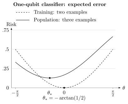
Exact expected errors of the stochastic measurement classifier. The dashed curve averages two training examples; the solid curve averages the three-point population. Their distinct minima arise from which examples are included, with no shot noise or optimizer failure. The training set here is chosen deterministically, so this calculation is not a probabilistic generalization guarantee.

At $\theta=\pi/3$,

$$\begin{aligned} \widehat R&=\frac14,\\ R&=\frac13+\frac{\sqrt3}{12}\approx0.477671,\\ R-\widehat R&=\frac{1+\sqrt3}{12}\approx0.227671. \end{aligned}$$

The deterministic classifier using the signs of the same exact scores instead has training error zero and population error $1/3$. Reporting one of these errors while implementing the other classifier would be incorrect.

Generalization and measurement precision

For a fixed predictor, population risk is $R(h)=\mathbb E_{\mathcal D}\ell(h(X),Y)$; empirical risk is the average over the observed training examples. Suppose the examples are iid, the loss is in $[0,1]$, and the finite class $\mathcal H$ is fixed independently of the sample. Hoeffding’s inequality and a union bound give, simultaneously for all $h\in\mathcal H$ with probability at least $1-\delta$,

$$|R(h)-\widehat R_m(h)| \le\sqrt{\frac{\log(2|\mathcal H|/\delta)}{2m}}.$$

Because the statement holds for the whole class, it also holds for a member selected using the training data. For a single predictor fixed independently of the evaluation sample, error tolerance $0.05$ and failure probability $0.05$, the sufficient count is $m=738$. This is a count of independent examples, not shots on one example. If $\widehat R$ itself is estimated from finite-shot circuit means, its additional estimation error must be included.

Continuous circuit families require a capacity bound rather than substituting an infinite class size into this expression. For fixed encodings, bounded observable losses and $T$ independently parameterized channels acting on a bounded number of qubits, Caro and collaborators obtain representative high-probability scaling

$$O\!\left(\sqrt{\frac{T\log(eT)}m}\right).$$

If each channel is reused at most $M$ times, the corresponding scaling is $O(\sqrt{T\log(eMT)/m})$, with constants and confidence terms suppressed. The number of independent trainable channels and the number of uses are different. Architecture selection also requires its own capacity term Caro et al. (2022).

A small gap does not ensure small risk if the training risk is large. These bounds also do not guarantee optimization, calibration or good predictions after the input distribution changes. Class imbalance can make overall accuracy misleading; class-specific errors and calibration answer additional questions.

Resolving a gradient

For a parameter appearing once in a Pauli rotation, the parameter-shift rule is

$$g=\partial_\theta f =\frac{f(\theta+\pi/2)-f(\theta-\pi/2)}2.$$

With $S$ independent outcomes in $[-1,1]$ at each shift, $\operatorname{Var}\widehat g\le1/(2S)$. Thus $S\ge z^2/(2g^2)$ is a sufficient worst-case condition for a signal of magnitude $|g|$ to be at least $z$ estimator standard deviations. It is not a necessary count, nor does “three standard deviations” itself imply a Gaussian tail probability.

A distribution-free alternative follows by applying Hoeffding to the $2S$ independent weighted outcomes. For nonzero $g$,

$$\Pr(\widehat g\text{ has the wrong sign or is zero}) \le e^{-Sg^2}.$$

These estimates concern measurement of a particular gradient. A small gradient may reflect a stationary point, an unsuitable encoding, or concentration under specific ansatz/noise assumptions. It does not by itself establish a barren plateau or poor generalization. The more general shift rules and trainability conditions are explained in variational algorithms.

A three-point kernel calculation

For $|\phi(x)\rangle=R_y(2x)|0\rangle$ and $x\in\{0,\pi/4,\pi/2\}$, the overlap is $\cos(x-x')$. Hence

$$K=\begin{pmatrix}1&1/2&0\\1/2&1&1/2\\0&1/2&1\end{pmatrix}.$$

Its antisymmetric eigenvector $(1,0,-1)^{\mathsf T}$ has eigenvalue one; the symmetric subspace gives $1\pm1/\sqrt2$. All eigenvalues are positive and their product is $1/2$. The corresponding SWAP probabilities are $1$, $3/4$ or $1/2$.

For pure one-qubit states, $\|\rho(x)-\rho(x')\|_F^2=2[1-k(x,x')]$. The projected kernel with $\gamma=1$ therefore has neighboring entries $a=e^{-1}$ and endpoint entry $b=e^{-2}$. Its determinant is

$$\det K_{\rm PQ}=1-2a^2+2a^2b-b^2\approx0.747645.$$

To turn a similarity matrix into a predictor, give the three inputs labels $y=(1,-1,1)^{\mathsf T}$. With $\lambda=1/2$, kernel ridge regression gives

$$a=\frac17(8,-10,8)^{\mathsf T},\qquad Ka=\frac17(3,-2,3)^{\mathsf T}.$$

All three fitted signs are correct, although regularization keeps the scores away from the labels. This finite fit says nothing yet about new examples. The following NumPy calculation also evaluates one new point:

import numpy as np

x = np.array([0.0, np.pi / 4, np.pi / 2])
states = np.array([[np.cos(t), np.sin(t)] for t in x])
K = np.abs(states @ states.T) ** 2
y = np.array([1.0, -1.0, 1.0])
a = np.linalg.solve(K + 0.5 * np.eye(3), y)
x_new = np.pi / 8
state_new = np.array([np.cos(x_new), np.sin(x_new)])
k_new = np.abs(states @ state_new) ** 2
print(K @ a)           # [3/7, -2/7, 3/7]
print(k_new @ a)       # (6 - 5*sqrt(2))/14

This small feature map is easy to compute classically. Its purpose is to show exactly where state preparation, overlap measurement and classical fitting enter a kernel method.

Born models and learning from quantum systems

A quantum circuit Born model defines

$$q_\theta(z)=|\langle z|U_\theta|0^n\rangle|^2.$$

Measurement supplies samples from $q_\theta$; it need not give an efficient exact evaluation of $q_\theta(z)$. A loss based on samples makes different demands from a likelihood requiring those probabilities. Coyle and collaborators study an Ising Born machine and conditional sampling hardness; hardness of sampling does not ensure that training finds a useful target distribution Coyle et al. (2020).

For a concrete two-qubit model, apply $R_y(2\theta)$ on the first qubit, then a CNOT from the first to the second. The state is $\cos\theta|00\rangle+\sin\theta|11\rangle$. It has $q(00)=\cos^2\theta$, $q(11)=\sin^2\theta$ and zero probability on $01,10$. For a target uniform on $00,11$, maximum mean discrepancy with the delta kernel $k(z,z')=\delta_{zz'}$ reduces to

$$\operatorname{MMD}^2(p,q)=\sum_z[p(z)-q(z)]^2 =\frac12\cos^2(2\theta).$$

At $\theta=\pi/8$ the loss is $1/4$ and its derivative is $-1$; at $\theta=\pi/4$ the generated distribution matches the target. Sampling a complicated state is unnecessary for this task.

Quantum data can create a different opportunity. A learner retaining quantum systems can perform joint measurements that are unavailable after every system has been separately measured and discarded. Huang and collaborators prove exponential sample separations for specified learning-from-experiments tasks under such access assumptions Huang et al. (2022). Related results distinguish predicting well on average under a fixed input distribution from predicting uniformly well on every input; the latter can require very different resources Huang, Kueng and Preskill (2021). These are statements about the permitted quantum experiments, not automatic speedups for a classical table of features.

When quantum computation changes learning cost

Hard simulation of a feature state does not imply hard prediction of its labels. A classical learner may exploit a few observable features, labels, low-rank structure or the geometry of the data without reconstructing the state. This distinction is central to the analysis of Huang and collaborators Huang et al. (2021).

Dequantization replaces a quantum subroutine with a classical algorithm under specified assumptions. Tang’s recommendation algorithm uses classical sample-and-query access analogous to the strong data access in the quantum proposal; it changes the comparison for that task, not for every learning problem Tang (2019). Rank, conditioning, approximation error and the requested output still matter. Conversely, Liu, Arunachalam and Temme construct a classical-data classification problem with a quantum kernel speedup conditional on the hardness of discrete logarithms Liu et al. (2021). The positive and negative results concern different assumptions and can both hold.

For a practical comparison, include input preparation, all training attempts, measurement repetitions and classical fitting. Separate training cost from the cost of another prediction:

$$C(A)=C_{\rm train}+A C_{\rm predict}.$$

A training advantage can differ from an inference advantage after many uses. State-preparation setup is similarly amortized only over the uses actually made. Noise can bias features or scores; mitigation may reduce bias while increasing sampling cost. Comparing methods at the same prediction error is more informative than comparing qubit counts alone.

Useful comparisons include simple predictors, well-tuned classical models and methods that exploit known structure. Bowles, Ahmed and Schuld discuss how model selection and classical baselines affect QML benchmarks Bowles et al. (2024). For experimental comparisons see algorithmic benchmarking; for changing research questions see quantum machine-learning frontiers.

Exercises

1. Information lost in an amplitude encoding

An encoder supplies only the amplitude states of $x=(1,2)$ and $x'=(2,4)$, with labels $-1$ and $+1$, respectively. Can any measurement classifier distinguish them? What is the minimum average error with equal prior probabilities? Explain why the number of qubits also does not determine generic loading time.

Solution

Both density operators are the same, because normalization removes the factor two. Every POVM has identical outcome probabilities on them, even with any fixed number of copies. With equal priors the minimum error is $1/2$. The norm or some other distinguishing feature must be supplied to solve this task. Separately, $\lceil\log_2N\rceil$ qubits can hold $N$ amplitudes, but an arbitrary complex pure state has $2N-2$ real parameters. Generic exact loading with bounded-size gates requires enough adjustable parameters to describe that family; logarithmic width does not give logarithmic preparation cost.

2. A positive training matrix and an impossible new feature

Prove $K_{ij}=\operatorname{Tr}(\rho_i\rho_j)$ is positive semidefinite. Then show that appending $(0.9,0.9)$ with self-overlap one to $K=I_2$ is inconsistent with any Gram representation, despite all entries lying in $[0,1]$.

Solution

For $A=\sum_i c_i\rho_i$, $c^\dagger Kc=\operatorname{Tr}(A^\dagger A)\ge0$. The proposed extended matrix has eigenvalues $1,1+0.9\sqrt2,1-0.9\sqrt2$; the last is negative. Its determinant is $1-2(0.9)^2=-0.62$. Thus valid individual ranges and a positive training matrix do not guarantee globally compatible similarities. Independent finite-shot errors must be considered at prediction time as well as fitting.

3. Stochastic and deterministic classifier errors

For the one-qubit worked classifier at $\theta=\pi/3$, calculate training and population risks for both the single-shot measurement label and the sign of the exact expectation. Find the angles minimizing the stochastic training and population risks.

Solution

The stochastic risks are $\widehat R=1/4$ and $R=1/3+\sqrt3/12$. The exact scores on the three inputs are $1/2,-\sqrt3/2,-1/2$; only the middle example has the wrong sign. Deterministic training error is therefore zero and population error is $1/3$. The training minimum is at $\theta=0$ modulo $2\pi$. Since $R'=\sin\theta/3+\cos\theta/6$, the population minimum is at $\theta=-\arctan(1/2)$ modulo $2\pi$, with value $1/2-\sqrt5/6$. These results use the explicitly chosen finite distribution, not an iid generalization theorem.

4. A two-qubit generator

Derive the state obtained by $R_y(2\theta)$ on qubit zero followed by $\mathrm{CNOT}_{0\to1}$, starting at $|00\rangle$. For a target uniform on $00,11$, derive its delta-kernel squared MMD and evaluate the loss and derivative at $\theta=\pi/8$.

Solution

The rotation gives $(\cos\theta|0\rangle+\sin\theta|1\rangle)|0\rangle$; CNOT changes the second term to $\sin\theta|11\rangle$. The two probabilities sum to one. Hence

$$\begin{aligned} \operatorname{MMD}^2 &=(1/2-\cos^2\theta)^2+(1/2-\sin^2\theta)^2\\ &=\frac12\cos^2(2\theta). \end{aligned}$$

At $\pi/8$ it is $1/4$; differentiation gives $-\sin4\theta=-1$ there.

5. A uniform generalization bound

For a fixed class of 20 predictors, iid examples, losses in $[0,1]$, $m=1000$ and $\delta=0.05$, calculate the uniform gap bound. What follows if the training-selected predictor has empirical risk $0.08$?

Solution

The gap is $\sqrt{\log800/2000}\approx0.057813$. With probability at least $0.95$ over the training sample, every predictor obeys the bound, so the selected predictor has $R\le0.137813$. This assumes the exact bounded losses used in the theorem; finite-shot estimates add their own error. The bound applies to the same population distribution. Without a further assumption, it gives no bound after an arbitrary distribution shift.

6. Gradient precision and a sign error bound

Two independent shifted means use $S$ shots each with outcomes in $[-1,1]$. For a gradient magnitude $g=0.02$, find a sufficient worst-case count for three standard deviations of separation. Separately find a count ensuring wrong-sign probability at most $0.05$ using the stated Hoeffding bound.

Solution

The variance criterion gives $S\ge9/[2(0.02)^2]=11250$ shots per shift, or 22500 preparations in total. It does not itself assign a Gaussian tail probability. The distribution-free sign bound gives $S\ge\log20/(0.02)^2$, whose ceiling is 7490 per shift. These are two different sufficient criteria. A smaller actual variance can reduce the count, while bias or dependent samples would require a different analysis.

7. Amortizing training cost

In common units, method Q costs $10000+2A$ and method C costs $100+5A$ for $A$ predictions. When is Q cheaper? If every Q prediction additionally requires input loading costing four units, does the crossover survive?

Solution

Without the extra loading, Q is cheaper when $9900<3A$, or $A>3300$. At 3300 the costs are equal. Including loading gives Q cost $10000+6A$, which exceeds $100+5A$ for every $A\ge0$. The prediction count and which operations must be repeated determine whether amortization helps.

8. A distinction invisible to local kernels

For $|\Phi_\pm\rangle=(|00\rangle\pm|11\rangle)/\sqrt2$, calculate the global overlap kernel and the projected kernel using both one-qubit reduced states. Can a classifier using only those local features identify the sign?

Solution

The global states are orthogonal, so $|\langle\Phi_+|\Phi_-\rangle|^2=0$. Tracing out either qubit gives $I/2$ for both signs. Every reduced-state distance vanishes, hence $k_{\rm PQ}(+,-)=1$. The local feature vectors are identical and cannot distinguish the signs. A joint observable can: $X\otimes X$ has expectation $+1$ on $|\Phi_+\rangle$ and $-1$ on $|\Phi_-\rangle$.

References

• J. Biamonte, P. Wittek, N. Pancotti, P. Rebentrost, N. Wiebe, and S. Lloyd, “Quantum machine learning,” Nature 549, 195–202 (2017), doi:10.1038/nature23474.
• J. Bowles, S. Ahmed, and M. Schuld, “Better than classical? The subtle art of benchmarking quantum machine learning models,” arXiv:2403.07059 (2024), doi:10.48550/arXiv.2403.07059.
• M. C. Caro, H.-Y. Huang, M. Cerezo, K. Sharma, A. Sornborger, L. Cincio, and P. J. Coles, “Generalization in quantum machine learning from few training data,” Nature Communications 13, 4919 (2022), doi:10.1038/s41467-022-32550-3.
• B. Coyle, D. Mills, V. Danos, and E. Kashefi, “The Born supremacy: quantum advantage and training of an Ising Born machine,” npj Quantum Information 6, 60 (2020), doi:10.1038/s41534-020-00288-9.
• L. Grover and T. Rudolph, “Creating superpositions that correspond to efficiently integrable probability distributions,” arXiv:quant-ph/0208112 (2002), arXiv:quant-ph/0208112.
• V. Havlíček, A. D. Córcoles, K. Temme, A. W. Harrow, A. Kandala, J. M. Chow, and J. M. Gambetta, “Supervised learning with quantum-enhanced feature spaces,” Nature 567, 209–212 (2019), doi:10.1038/s41586-019-0980-2.
• H.-Y. Huang, M. Broughton, J. Cotler, S. Chen, J. Li, M. Mohseni, H. Neven, R. Babbush, R. Kueng, J. Preskill, and J. R. McClean, “Quantum advantage in learning from experiments,” Science 376, 1182–1186 (2022), doi:10.1126/science.abn7293.
• H.-Y. Huang, M. Broughton, M. Mohseni, R. Babbush, S. Boixo, H. Neven, and J. R. McClean, “Power of data in quantum machine learning,” Nature Communications 12, 2631 (2021), doi:10.1038/s41467-021-22539-9.
• H.-Y. Huang, R. Kueng, and J. Preskill, “Information-theoretic bounds on quantum advantage in machine learning,” Physical Review Letters 126, 190505 (2021), doi:10.1103/PhysRevLett.126.190505.
• Y. Liu, S. Arunachalam, and K. Temme, “A rigorous and robust quantum speed-up in supervised machine learning,” Nature Physics 17, 1013–1017 (2021), doi:10.1038/s41567-021-01287-z.
• A. Pérez-Salinas, A. Cervera-Lierta, E. Gil-Fuster, and J. I. Latorre, “Data re-uploading for a universal quantum classifier,” Quantum 4, 226 (2020), doi:10.22331/q-2020-02-06-226.
• M. Schuld and N. Killoran, “Quantum machine learning in feature Hilbert spaces,” Physical Review Letters 122, 040504 (2019), doi:10.1103/PhysRevLett.122.040504.
• V. V. Shende, S. S. Bullock, and I. L. Markov, “Synthesis of quantum-logic circuits,” IEEE Transactions on Computer-Aided Design of Integrated Circuits and Systems 25, 1000–1010 (2006), doi:10.1109/TCAD.2005.855930.
• E. Tang, “A quantum-inspired classical algorithm for recommendation systems,” in Proceedings of the 51st Annual ACM SIGACT Symposium on Theory of Computing, 217–228 (2019), doi:10.1145/3313276.3316310.
• S. Thanasilp, S. Wang, M. Cerezo, and Z. Holmes, “Exponential concentration in quantum kernel methods,” Nature Communications 15, 5200 (2024), doi:10.1038/s41467-024-49287-w.