Quantum Algorithms for Optimization

Quantum optimization uses quantum operations to find a low-cost feasible answer, estimate an optimum, or sample useful candidates. These are different tasks. An algorithm that estimates a mean cost need not frequently produce an optimal bit string; one that estimates an optimal value need not return the corresponding vector.

The available input also matters. A reversible objective circuit, a searchable tree, a programmable Ising Hamiltonian and a convex-set membership oracle support different algorithms. This page explains how to choose among those possibilities through small calculations. Being NP-hard does not itself make a problem suitable for a quantum speedup.

Helpful background. Algorithmic primitives distinguishes quantum queries, state preparation and measured outputs; amplitude amplification explains coherent repetition; QAOA develops alternating cost and mixer operations.

Feasible answers and optimization guarantees

For a finite, nonempty feasible set $\mathcal F$, let

$$C^*=\min_{x\in\mathcal F}C(x).$$

Unless stated otherwise, lower cost is better. For continuous problems, existence of a minimizer needs justification: continuity on a nonempty compact set is one sufficient condition. Otherwise the appropriate quantity may be an infimum that no feasible point attains.

Three questions already lead to different outputs:

Question	Useful answer	What remains to check
Is there a feasible point below a threshold?	A candidate $x$ with $C(x)\le\tau$	Its constraints and cost
What is the optimum value?	A scalar estimate of $C^*$	Its error and confidence
Which point is optimal?	An optimizing point or bit string	Its feasibility and the guarantee of optimality

A bounded-error algorithm can return an exact optimizer with probability at least $1-\delta$ without attaching an efficiently checkable proof that this particular output is optimal. Its theorem gives the probability guarantee. A separately verifiable certificate is stronger output: for minimization, a feasible value $U$ together with a valid lower bound $L$ certifies

$$0\le U-C^*\le U-L.$$

Recomputing a candidate’s objective is usually much easier than excluding every better candidate. The best sample observed so far is not automatically an optimality certificate.

For a nonnegative maximization objective with optimum $V^*>0$, an approximation ratio $V(x)/V^*$ can be useful. Adding a constant preserves the optimizer but changes this ratio: values $1$ and $2$ have ratio $1/2$, whereas values $101$ and $102$ have ratio $101/102$. Use additive gaps when the zero of the objective is arbitrary. For nonnegative weighted MaxCut, the Goemans–Williamson algorithm provides a classical approximation guarantee worth comparing with quantum methods.

A mean cost is not a hit probability

Suppose the target is $C\le1$. A distribution concentrated at $C=2$ and a distribution split equally between $C=0$ and $C=4$ both have mean $2$. Their target probabilities are respectively $0$ and $1/2$. With $R$ independent samples the second succeeds at least once with probability $1-2^{-R}$, while the first never succeeds.

There can nevertheless be useful bounds from the mean. For a nonnegative integer cost with optimum $0$ and every nonoptimal cost at least $\Delta>0$,

$$\mathbb E[C]\ge\Delta(1-p_0), \qquad p_0\ge1-\frac{\mathbb E[C]}{\Delta}.$$

The bound is informative only when the mean is below the known gap. Without the range or gap assumption, it does not follow from a mean alone. Feasibility also matters: a very low cost on an infeasible string is not a good answer.

Binary costs, penalties and Ising Hamiltonians

A quadratic binary cost has the form

$$F(x)=c+\sum_iq_ix_i+\sum_{i<j}q_{ij}x_ix_j, \qquad x_i\in\{0,1\}.$$

Set $x_i=(1-z_i)/2$, where $z_i=\pm1$ is the eigenvalue of $Z_i$ on the computational state $\lvert x_i\rangle$. The resulting diagonal Hamiltonian satisfies $H_C\lvert x\rangle=F(x)\lvert x\rangle$. Keep its constant term when comparing energies, even though the constant does not change which strings minimize them.

When a penalty actually enforces a constraint

Write $F_P=F_0+PG$, where $G\ge0$ and $G=0$ precisely on the feasible set. Assume that this set is nonempty. Let $F_{\mathrm f}$ be its minimum, and suppose every infeasible string has $G(x)\ge g_{\min}>0$ and $F_{\mathrm f}-F_0(x)\le B$. Then

$$F_P(x)-F_{\mathrm f} \ge -B+Pg_{\min}>0$$

whenever $P>B/g_{\min}$. This sufficient condition concerns exact ground states; it does not say that a finite-temperature sampler, a shallow circuit or a noisy device outputs only feasible strings.

Increasing $P$ can also make a hardware implementation harder. If the largest coefficient is rescaled to a fixed physical limit, an order-one difference between feasible costs may shrink like $1/P$ relative to temperature or control errors. An exact algebraic penalty and a useful physical scale are separate considerations.

Worked example: three weighted vertices

On a triangle with vertex weights $(3,2,2)$, an independent set cannot select two adjacent vertices. Minimize

$$F_P(x)=-3x_0-2x_1-2x_2 +P(x_0x_1+x_1x_2+x_0x_2).$$

The best feasible string is $100$, with value $-3$. The possible competitors for the global minimum are

$$\begin{aligned} F_P(111)&=-7+3P,\\ F_P(101)=F_P(110)&=-5+P,\\ F_P(100)&=-3. \end{aligned}$$

For $P\ge0$, every other string lies above at least one of these. Thus the ground string is $111$ for $P<1$; $111,101,110$ tie at $P=1$; $101,110$ minimize for $1<P<2$; and $100,101,110$ tie at $P=2$. Only $P>2$ makes every ground string feasible.

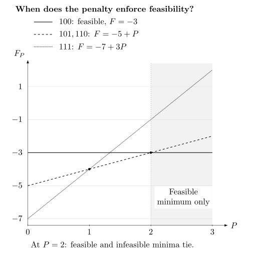
The three curves give the candidate ground energies of the weighted triangle. The lowest curve determines the answer. At $P=2$, feasibility is not assured because two infeasible strings remain degenerate with $100$.

At $P=4$, all eight values in order $000,001,\ldots,111$ are $(0,-2,-2,0,-3,-1,-1,5)$. Substituting the binary-to-spin relation gives

$$F_4(z)=-\frac12-\frac12z_0-z_1-z_2 +z_0z_1+z_1z_2+z_0z_2.$$

For example, $100$ maps to $(-1,+1,+1)$ and still has energy $-3$.

Coefficient precision can change the optimum

Suppose a programmed cost satisfies $\lvert\widetilde F(x)-F(x)\rvert\le\eta$ for every string. If $x^*$ is a true minimizer and $\widetilde x$ minimizes the programmed cost, then

$$F(\widetilde x)\le F(x^*)+2\eta.$$

The two error terms arise when comparing each cost to its programmed value. A unique optimum separated by a gap greater than $2\eta$ therefore remains the unique optimum. At equality a tie can occur. This is a uniform cost error bound, not a bound on one coefficient unless the contributions of all coefficients have been included. Ancilla reductions, physical chains and broken-chain repair need their own analysis.

Minimum finding and amplified proposals

For $N$ entries with coherent value and comparison access, the Dürr–Høyer algorithm finds an index of a minimum using $O(c\sqrt N)$ value queries, with failure at most $2^{-c}$. It improves an incumbent by searching for a smaller value. Strict improvement, or a specified tie-breaking order, avoids treating an equal-cost result as progress. This theorem counts queries, not the time to load an arbitrary table or build its reversible evaluation circuit.

For a fixed threshold, mark strings whose objective and feasibility tests both pass. If the initial success probability is $a$, the ideal Grover rotation gives

$$p_k=\sin^2((2k+1)\theta), \qquad \theta=\arcsin\sqrt a.$$

The derivation and unknown-$a$ schedules are in Grover search. More iterations are not always better: an excessive rotation can reduce success. The unstructured lower bounds and optimal search analysis refer to that oracle setting, not every structured optimization problem.

Worked example: a threshold and two attempts

Take the values

$$(13,4,9,1,7,12,2,10,6,3,11,15,5,14,8,0).$$

Values strictly below $3$ occur at zero-based indices $3,6,15$. Uniform preparation has $a=3/16$; one Grover iterate gives

$$p_1=\frac{243}{256}\approx0.949219.$$

Two independent, verified attempts succeed at least once with probability

$$1-(1-p_1)^2=\frac{65367}{65536}\approx0.997421.$$

This meets a $0.99$ target, while one attempt does not. The two attempts use two preparations, two phase queries and two diffusion operations. If each phase query computes a value, applies its threshold phase and uncomputes, it uses two value-oracle calls, giving four in total. Measurement and classical verification are additional operations.

Coherent use of a classical heuristic

If a classical randomized algorithm is given as a bounded-time circuit with explicit random bits, it can be made reversible while retaining those bits and its workspace. Prepare the random bits in superposition and run that circuit coherently. The resulting state need not be a pure state of the candidate register alone:

$$A\lvert0\rangle= \sum_r\sqrt{p(r)} \lvert r\rangle\lvert x(r)\rangle\lvert w(r)\rangle.$$

A success test on $x(r)$ and a reflection about the whole prepared state still permit amplitude amplification. Retained garbage is not by itself an obstacle: $A^\dagger$ reverses it. Discarding or measuring that workspace before the reflection changes the procedure and can destroy the interference.

A device that supplies only classical samples does not supply this coherent circuit or its inverse. Variable-time stopping, external memory calls and finite precision also affect the cost of reversible implementation. Once those operations are available, a proposal with target weight $a$ changes the ideal repetition scale from $1/a$ to $1/\sqrt a$, under the appropriate known- or unknown-success search scheme.

Structured search through graphs and trees

Structure can matter more than a flat search improvement. Dynamic programming, symmetry reduction, bounds or good variable ordering may avoid most of the $2^n$ candidate strings.

For example, let a finite reversible ergodic Markov chain have stationary distribution $\pi$, marked mass at least $\epsilon$, and absolute spectral gap $\delta>0$. A lazy chain avoids negative eigenvalues near $-1$. With coherent setup, update and marked-state checking costs $S,U,C$, the MNRS quantum search algorithm finds a marked state, when one exists under the promise, with constant success at cost

$$O\!\left[ S+\frac1{\sqrt\epsilon} \left(\frac{U}{\sqrt\delta}+C\right) \right].$$

A slow-mixing chain can make the update term large. The quantum-walk treatment explains the spectral construction.

For a backtracking tree with $T$ nodes on $n$ variables, Montanaro (2018) gives a bounded-error solution-finding procedure using $O(\sqrt T\,n^{3/2}\log n)$ tests under its coherent branching and predicate assumptions. The depth factors and reversible cost of each test matter.

Branch-and-bound also assigns a lower cost bound to each partial assignment. The bound must never exceed the cheapest feasible completion. An overestimated bound can prune the true optimum. A rounded lower bound needs a conservative error margin, not merely a small average numerical error.

In the bounded-degree tree model of Montanaro (2020), node bounds are nondecreasing down each branch, integer-valued in a known finite range, or infinite for an impossible branch. Let $d$ be the depth, $c_{\max}$ bound the finite cost range, and $T_{\min}$ count nodes remaining when bounds above the optimal cost are removed. A minimum-cost leaf can be found with constant failure probability using

$$\widetilde O\!\left( \sqrt{T_{\min}}\,d^{3/2}\log c_{\max} \right)$$

bound and branching queries. Logarithmic factors in depth, cost precision and inverse failure probability are suppressed. If there is no solution, $T_{\min}$ is the whole tree. The comparison uses the same branching and bounding procedures; its classical lower-bound comparison concerns finding all minimal leaves, or the usual distinct-cost case. It does not compare against every classical solver with different preprocessing.

Variational circuits, adiabatic evolution and annealing

These methods act on a cost Hamiltonian rather than only on a table of values. Their guarantees are different.

Method	How it uses the cost	What determines the result
QAOA	Alternates cost phases with a mixer	Initial state, mixer, depth and trained angles
Adiabatic computation	Follows an evolving low-energy subspace	Preparation, path, gap, schedule and runtime
Quantum annealing	Evolves under a programmed driver and cost	Finite-time dynamics, environment and decoding

For QAOA, with the first layer acting first, write

$$\lvert\psi_p\rangle= e^{-i\beta_pH_M}e^{-i\gamma_pH_C}\cdots e^{-i\beta_1H_M}e^{-i\gamma_1H_C}\lvert s\rangle.$$

Here $H_C$ represents a minimization cost. The MaxCut convention in the linked article instead maximizes a reward $V$: using $H_C=-H_V$ reverses the cost-phase sign at the same numerical angle. A constant shift adds only a global phase to an uncontrolled cost evolution.

A constraint-preserving mixer keeps a feasible initial state inside the feasible subspace. Connectivity of its transitions is an additional reachability question, not the definition of preservation; even connectivity alone does not prove that a fixed alternating ansatz can prepare every state. See the alternating-operator construction.

The ideal minimum of $\langle H_C\rangle$ over all angles, a trained parameter choice, its estimated mean and its measured best bit string are different. Training uses many circuit evaluations; independent samples should assess the selected parameters. Family-specific guarantees and low-depth obstructions are discussed with their assumptions on the QAOA page, rather than implying universal success or failure.

For an adiabatic path $H(s)=[1-A(s)]H_0+A(s)H_P$, require $A(0)=0$, $A(1)=1$ and a physical schedule $s(t)$. Endpoint ground states alone give no runtime bound. Relevant gaps, derivative couplings, smoothness and possible degeneracy enter the error estimate. The equivalence with gate computation established by Aharonov et al. does not give an efficient gap for an arbitrary optimization path.

Quantum annealing may be nonadiabatic and open to an environment; its final distribution need not be Gibbs or ground-state concentrated. Embedding, coefficient rescaling, readout, broken-chain repair and rejected samples all affect the rate of useful answers. The transverse-field approach originates in Kadowaki and Nishimori (1998).

Convex optimization and checkable bounds

For this section use a maximization linear program:

$$\begin{aligned} \text{primal:}\quad &\max_{x\ge0} c^Tx, &Ax&\le b,\\ \text{dual:}\quad &\min_{y\ge0} b^Ty, &A^Ty&\ge c. \end{aligned}$$

For feasible $x,y$, multiplying the inequalities by nonnegative coordinates gives $c^Tx\le x^TA^Ty\le b^Ty$. Thus a primal point gives a lower bound and a dual point an upper bound. Equality proves optimality without an enumeration of all points.

For a semidefinite program, replace $x\ge0$ by a positive semidefinite matrix $X\succeq0$, the objective by $\operatorname{Tr}(CX)$ and constraints by $\operatorname{Tr}(A_iX)\le b_i$. Its dual requires $\sum_i y_iA_i\succeq C$, $y_i\ge0$. Weak duality follows from positivity of the trace of the product of two positive matrices. Zero duality gap or attainment needs additional hypotheses, such as appropriate strict feasibility; it is not automatic for every SDP.

Worked example: one point and one bound

Maximize $3x+2y$ subject to $x,y\ge0$, $x+y\le4$, $x\le2$, $y\le3$. The feasible point $(2,2)$ has value $10$. Nonnegative dual multipliers $(u,v,w)=(2,1,0)$ satisfy $u+v\ge3$, $u+w\ge2$ and give

$$3x+2y\le2(x+y)+x\le2(4)+2=10.$$

The matching lower and upper bounds prove that $(2,2)$ is optimal.

Numerical residuals cannot be ignored. Multipliers $(1.99,1,0)$ would give the false upper bound $9.96$, because both dual constraints have deficit $0.01$. If all primal feasible points satisfy $\lVert x\rVert_1\le R_x$, an approximate nonnegative dual vector gives the rigorous bound

$$c^Tx\le b^Ty+ R_x\lVert(c-A^Ty)_+\rVert_\infty.$$

Here $(\cdot)_+$ takes positive parts coordinatewise. In the example $x+y\le4$ gives $R_x=4$, so the corrected bound is $9.96+0.04=10$. The correction requires a valid radius bound and controlled arithmetic.

Which operations are actually supplied?

A membership oracle says whether a point belongs to a convex body, up to a specified boundary tolerance. A separation oracle supplies a hyperplane excluding an exterior point. Coherent membership, entry access to a sparse matrix and a block encoding are distinct inputs.

Under geometric and precision assumptions including inner/outer radius bounds, van Apeldoorn and collaborators implement separation with polylogarithmically many quantum membership queries and optimization in dimension $d$ with $\widetilde O(d)$ such queries. The latter improves a quadratic classical upper bound; it is not a matching quadratic separation theorem. Their optimization lower bounds are $\Omega(\sqrt d)$ queries with a known interior point and $\Omega(d)$ separation queries without one van Apeldoorn et al. (2020). Returning a hyperplane or optimizer explicitly still requires writing its coordinates; a query bound does not count that output time.

For entry-query LP/SDP solvers, a separate worst-case bound becomes $\Omega(mn)$ when constraint count $m$ and matrix dimension $n$ are comparable. The constructed hard family has growing primal and dual solution-size parameters: it is not a lower bound with every norm and accuracy parameter fixed. In that construction the customary bounds $R,r$ grow as $\Theta(\min\{m,n\}^2)$ at constant additive accuracy van Apeldoorn et al. (2020), Corollary 31. Dependence on $Rr/\epsilon$, sparsity and the output must accompany any dimension-based comparison.

A quantum state over $4096$ basis labels needs a $12$-qubit register, but does not reveal $4096$ signed coordinates in one measurement. An explicit vector using $24$ bits per coordinate contains $98{,}304$ bits, or $12$ KiB. These are different answers. The payload count alone is not a universal tomography or query lower bound. Quantum linear algebra and block encodings explain the relevant implicit representations.

Repetitions and the cost of a useful answer

Let $p$ be the probability that an attempt returns a verified target. For independent identically distributed attempts and $0<p<1$, the smallest number reaching failure at most $0<\delta<1$ is

$$R=\left\lceil\frac{\ln\delta}{\ln(1-p)}\right\rceil.$$

If $p=0$, repetition cannot help; if $p=1$, one attempt suffices. If samples share a random device condition, identical one-run probabilities do not establish independence. In the extreme case where one Bernoulli variable determines every run, repeating leaves the success probability at $p$ rather than raising it to $1-(1-p)^R$.

For adaptive attempts let $q_j$ be the probability of success on attempt $j$, conditional on all previous attempts failing. Then the exact failure probability is $\prod_j(1-q_j)$. Uniform conditional lower bounds $q_j\ge p_{\min}$ give a conservative iid-shaped bound even without independence. Marginal one-run probabilities cannot be substituted for these conditional quantities.

Postselection also changes the count. If feasibility acceptance is $f$ and the conditional target probability among accepted strings is $q$, the per-preparation target probability is $p=fq$. At $f=0.1$, $q=0.9$, a $99\%$ success target requires $49$ independent preparations, not the two suggested by using $q$ alone. All discarded samples took time.

A pilot estimate of $p$ has uncertainty. If $p_L$ is a valid lower confidence bound with failure $\alpha$, choosing the repetitions from $p_L$ and a retry failure target $\beta$ bounds the combined failure by $\alpha+\beta$, provided the future attempts obey the assumed success model.

Finally compare complete procedures: input preparation, reversible work, training, repetitions, readout and verification. Use classical methods suited to the same structure—bounds, relaxations, dynamic programming and tuned heuristics, not only uniform guessing. Practical comparisons and definitions of speedup are discussed by Rønnow et al. and in optimization case studies; algorithmic benchmarking explains how to compare the same output quality and confidence.

Exercises

1. Convert a binary polynomial

For $F(x)=2-5x_0+3x_1+6x_0x_1$, find the Ising constant, fields and pair coupling. Check every bit string.

Solution

Substituting $x_i=(1-z_i)/2$ gives

$$F(z)=\frac52+z_0-3z_1+\frac32z_0z_1.$$

The constant is $2-5/2+3/2+6/4=5/2$; the fields are $5/2-6/4=1$ and $-3/2-6/4=-3$. In order $00,01,10,11$, both formulas give $(2,5,-3,6)$. Omitting the constant preserves the minimizing string but changes every energy.

2. Test a borderline penalty

Minimize $F_0=-4x_0-3x_1$ with $x_0+x_1\le1$, using penalty $PG=P x_0x_1$. For which $P$ are all ground strings feasible?

Solution

The feasible strings have values $0,-3,-4$. The infeasible string $11$ has value $-7+P$. It must lie strictly above $-4$, so $P>3$. At $P=3$, feasible $10$ and infeasible $11$ tie. Requiring only that some ground state be feasible would miss this distinction.

3. Bound the ground-string probability

A nonnegative integer cost takes values $0,2,5$ and has mean $0.6$. Find the strongest lower bound on the probability of cost zero that follows from the smallest positive cost. Give a distribution attaining it.

Solution

Since $\mathbb E[C]\ge2(1-p_0)$, $p_0\ge0.7$. The distribution $(p_0,p_2,p_5)=(0.7,0.3,0)$ attains equality. Probability at cost $5$ would need more weight at zero to keep the same mean. The exact optimum probability is not fixed by the mean.

4. Count independent threshold searches

Derive $p_1=243/256$ for the sixteen-entry example and find the smallest number of independent attempts for $99\%$ confidence.

Solution

With $\sin\theta=\sqrt3/4$, $\sin3\theta=3\sqrt3/4-3\sqrt3/16=9\sqrt3/16$. Squaring gives $243/256$. One attempt falls short; two give $1-(13/256)^2=65367/65536\approx0.997421$. They require two threshold phase queries, or four value queries if each phase operation computes and uncomputes its value.

5. Compare flat and tree search costs

Compare $\sqrt N$ for $N=2^{40}$ with the displayed backtracking expression $\sqrt T\,d^{3/2}\log_2d$ for $T=2^{18}$, $d=40$. Let one flat query cost $q_v$ gates and one coherent tree test cost $q_t$. When is the latter displayed expression smaller?

Solution

The values are $2^{20}=1{,}048{,}576$ and approximately $6.89\times10^5$. The displayed tree cost is smaller if $q_t<1.52q_v$. This compares only those leading expressions; asymptotic notation hides constants, and the branching procedure determines $T$. It is not a measured crossover or a comparison with the best classical algorithm.

6. Prove a linear-program optimum

For the linear program above, derive weak duality directly and use the primal point $(2,2)$ and dual point $(2,1,0)$ to prove optimality.

Solution

For feasible points and nonnegative dual variables,

$$\begin{aligned} 3x+2y &\le(u+v)x+(u+w)y\\ &=u(x+y)+vx+wy\\ &\le4u+2v+3w. \end{aligned}$$

Both chosen points are feasible, and their objectives equal $10$. No primal point can do better and no dual point can give a smaller bound. This proves optimality without relying on the success of a numerical solver.

7. Repair a nearly feasible dual bound

In the same program, take $(u,v,w)=(2,0.98,0)$. Its raw objective is $9.96$. Bound the effect of its dual-constraint violation, first using $x+y\le4$, then the tighter individual constraint $x\le2$.

Solution

The deficits are $3-(u+v)=0.02$ and $2-(u+w)=0$. The $\ell^1$ bound gives $9.96+4(0.02)=10.04$. Only the $x$ coefficient is deficient, so using $x\le2$ improves this to $9.96+2(0.02)=10$. Both corrected values are upper bounds; $9.96$ is not.

8. Include rejected samples

A sampler accepts a feasible answer with probability $0.1$; conditionally, $90\%$ of accepted answers meet the target. Compute the independent preparation count for $99\%$ confidence. Explain why the same marginal probabilities do not suffice when every preparation shares one random outcome.

Solution

One preparation succeeds with probability $0.09$. Thus $R=\lceil\ln(0.01)/\ln(0.91)\rceil=49$; $48$ do not suffice. Using the conditional probability $0.9$ would incorrectly give $2$. If the entire batch is determined by one Bernoulli success variable, the probability of any success is still $0.09$, however large the batch. The product formula instead needs probabilities conditional on previous failures, or a justified independence model.

References

• Dorit Aharonov, Wim van Dam, Julia Kempe, Zeph Landau, Seth Lloyd, and Oded Regev, “Adiabatic Quantum Computation Is Equivalent to Standard Quantum Computation,” SIAM Journal on Computing 37(1), 166–194 (2007), doi:10.1137/S0097539705447323.
• Charles H. Bennett, Ethan Bernstein, Gilles Brassard, and Umesh Vazirani, “Strengths and Weaknesses of Quantum Computing,” SIAM Journal on Computing 26(5), 1510–1523 (1997), doi:10.1137/S0097539796300933.
• Gilles Brassard, Peter Høyer, Michele Mosca, and Alain Tapp, “Quantum Amplitude Amplification and Estimation,” Contemporary Mathematics 305, 53–74 (2002), doi:10.1090/conm/305/05215.
• Christoph Dürr and Peter Høyer, “A Quantum Algorithm for Finding the Minimum,” arXiv:quant-ph/9607014 (1996), arXiv:quant-ph/9607014.
• Edward Farhi, Jeffrey Goldstone, and Sam Gutmann, “A Quantum Approximate Optimization Algorithm,” arXiv:1411.4028 (2014), arXiv:1411.4028.
• Michel X. Goemans and David P. Williamson, “Improved Approximation Algorithms for Maximum Cut and Satisfiability Problems Using Semidefinite Programming,” Journal of the ACM 42(6), 1115–1145 (1995), doi:10.1145/227683.227684.
• Lov K. Grover, “A Fast Quantum Mechanical Algorithm for Database Search,” Proceedings of the Twenty-Eighth Annual ACM Symposium on Theory of Computing, 212–219 (1996), doi:10.1145/237814.237866.
• Stuart Hadfield, Zhihui Wang, Bryan O’Gorman, Eleanor G. Rieffel, Davide Venturelli, and Rupak Biswas, “From the Quantum Approximate Optimization Algorithm to a Quantum Alternating Operator Ansatz,” Algorithms 12(2), 34 (2019), doi:10.3390/a12020034.
• Tadashi Kadowaki and Hidetoshi Nishimori, “Quantum Annealing in the Transverse Ising Model,” Physical Review E 58, 5355–5363 (1998), doi:10.1103/PhysRevE.58.5355.
• Frédéric Magniez, Ashwin Nayak, Jérémie Roland, and Miklos Santha, “Search via Quantum Walk,” SIAM Journal on Computing 40(1), 142–164 (2011), doi:10.1137/090745854.
• Ashley Montanaro, “Quantum-Walk Speedup of Backtracking Algorithms,” Theory of Computing 14(15), 1–24 (2018), doi:10.4086/toc.2018.v014a015.
• Ashley Montanaro, “Quantum Speedup of Branch-and-Bound Algorithms,” Physical Review Research 2, 013056 (2020), doi:10.1103/PhysRevResearch.2.013056.
• Troels F. Rønnow, Zhihui Wang, Joshua Job, Sergio Boixo, Sergei V. Isakov, David Wecker, John M. Martinis, Daniel A. Lidar, and Matthias Troyer, “Defining and Detecting Quantum Speedup,” Science 345(6195), 420–424 (2014), doi:10.1126/science.1252319.
• Joran van Apeldoorn, András Gilyén, Sander Gribling, and Ronald de Wolf, “Convex Optimization Using Quantum Oracles,” Quantum 4, 220 (2020), doi:10.22331/q-2020-01-13-220.
• Joran van Apeldoorn, András Gilyén, Sander Gribling, and Ronald de Wolf, “Quantum SDP-Solvers: Better Upper and Lower Bounds,” Quantum 4, 230 (2020), doi:10.22331/q-2020-02-14-230.
• Christof Zalka, “Grover’s Quantum Searching Algorithm Is Optimal,” Physical Review A 60, 2746–2751 (1999), doi:10.1103/PhysRevA.60.2746.