Adiabatic Quantum Computation

Adiabatic quantum computation encodes a problem in the low-energy states of a Hamiltonian and approaches those states by changing the Hamiltonian gradually. The starting ground state should be easy to prepare; measuring the final state should yield a useful answer. The central question is how slowly the change must occur, at a fixed energy scale, to obtain that answer reliably. This page treats finite-dimensional closed systems; quantum annealing also considers finite-time and open-system processes.

Helpful background. Adiabatic approximation supplies instantaneous eigenstates and transition amplitudes. The circuit model supplies registers, measurements and computational resources.

Hamiltonian paths and encoded answers

For an instance $x$, choose a Hermitian path $H_x(s)$ with $0\leq s\leq1$. A schedule $s(t)$ specifies its physical traversal:

$$i\hbar\frac{d}{dt}|\psi_x(t)\rangle =H_x(s(t))|\psi_x(t)\rangle, \qquad s(0)=0,\quad s(T)=1.$$

The common interpolation

$$H_x(s)=(1-s)H_{{\rm i},x}+sH_{{\rm f},x}$$

is one choice. Additional terms or curved paths can change the spectrum even when the endpoints remain fixed. The path and the schedule are different: the same sequence of Hamiltonians can be traversed at different speeds.

For a classical cost function $C_x(z)$, a diagonal problem Hamiltonian is

$$H_{{\rm f},x}=\sum_z C_x(z)|z\rangle\langle z|.$$

Its ground states represent minimizing bit strings. Computational-basis measurement returns a candidate; the acceptance rule might require the exact minimum or allow a stated approximation. Penalties can exclude invalid configurations, but their coefficients and required precision count toward the cost. Preparing the ground state of $H_{{\rm i},x}$ must not hide the original hard problem.

More general encodings use a final subspace rather than one string. Projection into that subspace, preservation of a logical superposition within it, and production of a particular measurement distribution are distinct goals. In each case the measurement and classical decoding determine success.

The evolution is

$$U_x(T)=\mathcal T\exp\!\left[-\frac{i}{\hbar} \int_0^T H_x(s(t))\,dt\right].$$

Time ordering matters when Hamiltonians at different times fail to commute. Knowing the endpoint ground states alone does not determine the final state.

Spectral isolation and the relevant gap

For the usual gapped subspace theorem, follow a smooth spectral projector $P_x(s)$ of fixed rank along the whole path. Let $Q_x(s)=I-P_x(s)$. Its external gap is

$$g_x(s)=\operatorname{dist}\!\left( \operatorname{spec}(H_x|_{\operatorname{Ran}P_x}), \operatorname{spec}(H_x|_{\operatorname{Ran}Q_x})\right), \qquad g_{\min}=\min_{0\leq s\leq1}g_x(s).$$

For a nondegenerate ground state, this is $E_1-E_0$. For an isolated band containing several accepted states, degeneracies within the band do not close its external gap. But if a rank-one ground state merges with other states at the endpoint, one cannot merely enlarge $P(1)$ and apply the same fixed-rank theorem. One must choose a consistently isolated larger band, analyze the closing gap separately, or use another result.

An exactly conserved symmetry can restrict evolution to one sector. A state prepared there may experience a larger sector gap than the full-space gap. This simplification requires the entire Hamiltonian path to preserve the sector. If a perturbation breaks the symmetry, examine the perturbed full-space spectrum and couplings. Even the unperturbed full-space gap is not automatically a bound for that new problem. For a separated ordered band and a Hermitian perturbation of norm at most $\delta$, eigenvalue perturbation bounds give the useful estimate

$$g_{\mathrm{perturbed}}(s)\geq g_{\mathrm{unperturbed}}(s)-2\delta,$$

when the right side is positive. Smoothness and derivative bounds are still needed to control the perturbed dynamics.

For a fixed smooth path with a uniform gap, standard adiabatic theorems bound leakage as the traversal time increases. The constants depend on the gap and derivatives; a family of larger problems requires bounds on that dependence. A positive gap in one small matrix is not an efficient algorithm for arbitrary input sizes. See the adiabatic theorem for precise hypotheses and Jansen, Ruskai and Seiler for explicit gap-dependent estimates.

Choosing a schedule and measuring success

For a nondegenerate two-level path, define

$$M(s)=|\langle1(s)|H'(s)|0(s)\rangle|, \qquad \eta(t)=\frac{\hbar|\dot s(t)|M(s)}{\Delta(s)^2}.$$

This local ratio estimates where transitions are difficult to suppress. It is a schedule-design diagnostic, not a universal error bound. Where $M(s)>0$, holding it at $\epsilon$ suggests

$$\dot s=\frac{\epsilon\Delta(s)^2}{\hbar M(s)}, \qquad T=\frac{\hbar}{\epsilon}\int_0^1\frac{M(s)}{\Delta(s)^2}\,ds.$$

A zero of $M$ does not permit an infinite physical speed without further analysis; control limits or a separately justified schedule must handle that region. Endpoint behavior and regularity also matter. Neither this construction nor the minimum gap alone proves an assumption-free law $T\propto g_{\min}^{-2}$.

For an initial state in $P_x(0)$, the operator norm

$$\epsilon_{\mathrm{ad}}(T)=\|Q_x(1)U_x(T)P_x(0)\|$$

bounds the leakage amplitude for every normalized state in that initial subspace. If success means the final measurement accepts the whole band, failure probability is at most $\epsilon_{\mathrm{ad}}^2$. If a particular logical vector or decoded subset is required, population remaining in the band may still give a wrong answer.

More generally, for initial state $\rho_{0,x}$, measurement effects $M_y$ and accepted outcomes $\mathcal A_x$,

$$p_{\mathrm{succ}}(x)=\sum_{y\in\mathcal A_x} \operatorname{Tr}\!\left[M_yU_x(T)\rho_{0,x}U_x(T)^\dagger\right].$$

Independent repetitions with $0<p_{\mathrm{succ}}<1$ produce at least one successful outcome with probability $1-(1-p_{\mathrm{succ}})^R$. Thus a desired probability $\eta$ requires

$$R_\eta=\left\lceil\frac{\ln(1-\eta)}{\ln(1-p_{\mathrm{succ}})}\right\rceil.$$

Using this as an answer-selection procedure requires a verifier or another justified decoding rule. Repetition alone does not identify which unknown output is correct. Preparation, readout and reset costs recur along with the coherent evolution time.

A one-qubit interpolation

Set $\hbar=1$ and take

$$H_B=\frac{I-X}{2},\qquad H_P=\frac{I-Z}{2}, \qquad H(s)=(1-s)H_B+sH_P.$$

The initial ground state is $|+\rangle$ and the final ground state is $|0\rangle$. The instantaneous eigenvalues are

$$E_\pm(s)=\frac{1\pm\Delta(s)}2, \qquad \Delta(s)=\sqrt{(1-s)^2+s^2}.$$

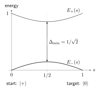
The ground state changes from $|+\rangle$ to $|0\rangle$ while its energy remains separated from the excited level. The gap is smallest at $s=1/2$, but the final success probability also depends on the traversal schedule.

For the linear schedule $s=t/8$, direct Schrödinger evolution in the order $(|0\rangle,|1\rangle)$ gives

$$|\psi(8)\rangle\approx{} (0.804636102344-0.581531139378i)|0\rangle +(-0.078388950073+0.090760394695i)|1\rangle.$$

Consequently $p_0\approx0.9856177233$ and $p_1\approx0.0143822767$. Keeping the identity term in $H$ fixes the displayed common phase. An independent ODE integration and a refined product of midpoint matrix exponentials check these values; no measurement sampling is involved.

The derivative coupling is $M(s)=1/[2\Delta(s)]$, so

$$\Delta_{\min}=\frac1{\sqrt2}, \qquad \eta_{\max}=\frac{\sqrt2}{8}\approx0.176777.$$

The diagnostic and $1-p_0$ are different quantities. This small example makes the distinction visible: spectral information guides a schedule, while direct evolution answers the finite-time measurement question. It does not establish scaling with problem size.

From circuit histories to Hamiltonian ground states

A circuit $U_L\cdots U_1$ can be represented by a data register and a clock. Its history state is

$$|\eta\rangle=\frac1{\sqrt{L+1}}\sum_{\ell=0}^L U_\ell\cdots U_1|\psi_{\mathrm{in}}\rangle\otimes|\ell\rangle_c, \qquad U_0=I.$$

The clock labels which prefix of the computation has been applied. A propagation Hamiltonian penalizes inconsistent neighboring slices:

$$H_{\mathrm{prop}}=\frac12\sum_{\ell=1}^L\bigl[ I\otimes(|\ell\rangle\langle\ell|+|\ell-1\rangle\langle\ell-1|) -U_\ell\otimes|\ell\rangle\langle\ell-1| -U_\ell^\dagger\otimes|\ell-1\rangle\langle\ell|\bigr].$$

Each term is positive semidefinite and annihilates the history state. A full construction also fixes the input, restricts the clock to valid configurations, supplies an easy initial state and proves a suitable gap along the interpolation. Without these additions, the propagation kernel alone does not implement the computation.

Measuring the unpadded clock gives the final time with probability $1/(L+1)$. Appending identity gates increases the fraction of clock positions that carry the final data state. The polynomial equivalence established by Aharonov and colleagues uses uniform constructions with bounded locality and controlled energy, precision and runtime overhead. It does not imply equal running times or make every optimization interpolation efficient. Hamiltonian simulation explains the other direction: implementing sufficiently well-specified Hamiltonian evolution with circuits.

A one-gate history

For $U=X$, order the registers as data then clock and choose

$$H_{\mathrm{start}}=I-|00\rangle\langle00|, \qquad H_{\mathrm{hist}}=\frac12(I-X_dX_c)+|10\rangle\langle10|.$$

The first ground state is $|00\rangle$. The second is

$$|\eta\rangle=\frac{|00\rangle+|11\rangle}{\sqrt2}, \qquad H_{\mathrm{hist}}|\eta\rangle=0.$$

Clock outcome one occurs with probability $1/2$ and then the data is certainly one, as required by $X|0\rangle=|1\rangle$.

Along $H(s)=(1-s)H_{\mathrm{start}}+sH_{\mathrm{hist}}$, even and odd parity form invariant blocks. Their eigenvalues are

$$\lambda_{A,\pm}(s)=\frac{1\pm\sqrt{(1-s)^2+s^2}}2, \qquad \lambda_{B,\pm}(s)=1\pm\frac{s}{\sqrt2}.$$

The full-space minimum ground-state gap is $1-1/\sqrt2\approx0.292893$, attained at $s=1$. The even sector containing the prepared state has minimum gap $1/\sqrt2$, attained at $s=1/2$. These values answer different questions; a symmetry-breaking perturbation requires a new full-space analysis. No schedule has been specified here, so the endpoint eigenstate and gap calculations do not determine finite-time preparation success.

Energy scales, implementation and limitations

If $\widetilde H(s)=aH(s)+b(s)I$ with $a>0$, the eigenvectors remain the same and energy differences scale by $a$. Traversing the rescaled path with $\widetilde s(t')=s(at')$ reproduces the same ray in time $T/a$, with an additional scalar phase from $b(s)$. This faster evolution uses proportionally larger nonidentity coefficients and a faster schedule. The operator norm itself also depends on the chosen scalar offset; the spectral range does not.

An efficient family must account for register size, interaction locality, term count, coefficient magnitude and precision, preparation, traversal, measurement and classical decoding. Access to a symbolic path does not automatically provide its physical implementation or its controlled propagator.

Numerical propagation should be checked by step refinement and independent methods where possible; norm preservation alone does not bound state error. The time-propagation methods explain those checks. A finite path should not be assigned an infinite-sweep Landau–Zener probability without matching the sweep assumptions.

A closed-system theorem also does not establish thermal robustness or fault tolerance. Dissipation can both remove and create excitations; quantum annealing treats such regimes. Claims about computational advantage additionally need a specified task and a suitable classical comparison, as discussed in algorithmic benchmarking.

Exercises

Encode a Two-Bit Cost Function

For bits $x_1,x_2\in\{0,1\}$, encode

$$C(x_1,x_2)=2x_1+x_2+x_1x_2$$

as a diagonal two-qubit problem Hamiltonian using $x_j=(1-Z_j)/2$. Verify every computational-basis energy and state exactly what the calculation does not establish.

Solution

Substitution gives

$$\begin{aligned} H_P ={}&2\frac{I-Z_1}{2} +\frac{I-Z_2}{2} +\frac{(I-Z_1)(I-Z_2)}{4}\\ ={}& \frac74I -\frac54Z_1 -\frac34Z_2 +\frac14Z_1Z_2. \end{aligned}$$

In computational order:

• $|00\rangle$ has $(Z_1,Z_2)=(+1,+1)$ and energy $0$;
• $|01\rangle$ has $(+1,-1)$ and energy $1$;
• $|10\rangle$ has $(-1,+1)$ and energy $2$; and
• $|11\rangle$ has $(-1,-1)$ and energy $4$.

Thus the ordered spectrum is $\{0,1,2,4\}$, matching the four classical costs. The calculation establishes an endpoint encoding only. It supplies no initial Hamiltonian, path, gap, runtime, output-confidence analysis, or speedup.

Rescale the Hamiltonian and runtime

Let

$$\widetilde H(s)=aH(s)+b(s)I, \qquad a>0.$$

Given an original schedule $s(t)$ on $0\leq t\leq T$, find the schedule that reproduces the same final ray in time $T/a$, derive the extra phase, and identify the resources changed by the transformation.

Solution

Set $t'=t/a$ and compress the schedule as

$$\widetilde s(t')=s(at'), \qquad 0\leq t'\leq\frac{T}{a}.$$

If $|\psi(t)\rangle$ solves the original equation, then $|\psi(at')\rangle$ obeys

$$i\hbar\frac{d}{dt'}|\psi(at')\rangle = aH(s(at'))|\psi(at')\rangle.$$

The scalar term commutes with every operator and contributes only

$$\exp\!\left[ -\frac{i}{\hbar} \int_0^{T/a} b\!\left(\widetilde s(t')\right)\,dt' \right].$$

Therefore the final ray agrees with the original one. The statement is false for a general unchanged physical-time schedule, because the two evolutions then visit different path points at corresponding times.

The projectors are unchanged. All gaps, the spectral range, and nonidentity coefficients scale by $a$. The operator norm need not: the scalar shift changes the absolute eigenvalues. For example, $H=Z$, $a=2$, and $b=10$ give $\|2Z+10I\|=12$, although $2\|Z\|=2$. The compressed schedule requires proportionally faster control. These energy, coefficient-precision, bandwidth, and timing resources must be counted; $b(s)$ is phase-only for an isolated evolution but may matter under controlled evolution or phase-sensitive comparison.

Derive the Linear One-Qubit Gap

For the Hamiltonian in the linear one-qubit example, derive the eigenvalue gap, its minimum, the derivative coupling $|\langle1|H'|0\rangle|$, and the maximum local diagnostic at $T=8$.

Solution

The Hamiltonian is

$$H(s) = \frac12 \left[ I-(1-s)X-sZ \right].$$

Its nonidentity Bloch vector has length

$$\Delta(s)=\sqrt{(1-s)^2+s^2},$$

so

$$E_\pm(s)=\frac{1\pm\Delta(s)}{2}.$$

Minimizing $\Delta(s)^2=1-2s+2s^2$ gives $s=1/2$ and

$$\Delta_{\min}=\frac{1}{\sqrt2}.$$

For a two-level Bloch Hamiltonian, the off-diagonal derivative component is the part of the derivative perpendicular to the instantaneous Bloch vector. Here this gives

$$\left|\langle1(s)|H'(s)|0(s)\rangle\right| = \frac{1}{2\Delta(s)}.$$

With $\dot s=1/8$, the diagnostic is

$$\frac{|\dot s|}{2\Delta(s)^3}.$$

It is largest where the gap is smallest, so

$$\eta_{\max} = \frac18 \frac{1}{2(1/\sqrt2)^3} = \frac{\sqrt2}{8}.$$

This is a local diagnostic, not a theorem-level error bound.

Compare Linear and Local Schedules

For the same one-qubit path, evaluate

$$\int_0^1 \frac{|\langle1|H'|0\rangle|}{\Delta^2}\,ds$$

and compare the diagnostic runtimes for a constant-local-diagnostic schedule and a linear schedule at the same maximum diagnostic $\epsilon$.

Solution

Because $|\langle1|H'|0\rangle|=1/(2\Delta)$,

$$\int_0^1 \frac{|\langle1|H'|0\rangle|}{\Delta^2}\,ds = \int_0^1\frac{ds}{2\Delta^3}.$$

Let $u=2s-1$. Then $ds=du/2$ and $\Delta^2=(1+u^2)/2$, so

$$\begin{aligned} \int_0^1\frac{ds}{2\Delta^3} &= \frac{1}{\sqrt2} \int_{-1}^{1} \frac{du}{(1+u^2)^{3/2}}\\ &= \frac{1}{\sqrt2} \left[ \frac{u}{\sqrt{1+u^2}} \right]_{-1}^{1} =1. \end{aligned}$$

Holding the local diagnostic at $\epsilon$ gives

$$\dot s = \frac{\epsilon\Delta^2}{M} =2\epsilon\Delta^3,$$

and therefore

$$T_{\mathrm{local}} = \int_0^1\frac{ds}{2\epsilon\Delta^3} = \frac{1}{\epsilon}.$$

For a linear schedule, $\dot s=1/T$ and the maximum diagnostic is $\sqrt2/T$, so

$$T_{\mathrm{linear}}=\frac{\sqrt2}{\epsilon}.$$

This compares two uses of the same diagnostic. Neither equality is a general theorem relating runtime to actual adiabatic error.

Use an External Gap for a Degenerate Target

Consider

$$H_P=\frac{I+Z_1Z_2}{2}.$$

Identify its ground space, compare the sorted $E_1-E_0$ value with the external target-to-complement gap, and explain which one belongs in a subspace adiabatic theorem.

Solution

$Z_1Z_2$ has eigenvalue $+1$ on even-parity states $|00\rangle,|11\rangle$ and $-1$ on odd-parity states $|01\rangle,|10\rangle$. Hence

$$H_P|00\rangle=|00\rangle, \qquad H_P|11\rangle=|11\rangle,$$

while

$$H_P|01\rangle=0, \qquad H_P|10\rangle=0.$$

The accepted ground projector is

$$P = |01\rangle\langle01| +|10\rangle\langle10|.$$

The ordered spectrum is $\{0,0,1,1\}$. Consequently the naive sorted gap is

$$E_1-E_0=0,$$

because it measures an internal degeneracy within the accepted band. The distance from that band to the rejected even-parity space is instead

$$g_{\mathrm{external}}=1.$$

The external value belongs in a theorem or leakage statement that transports the whole accepted subspace. If a task distinguishes coherent vectors inside the odd-parity space, internal splitting and logical transport require additional analysis.

Pad a History State

A circuit contains $L=3$ nonidentity gates and is followed by $r=5$ identity gates. For the uniform history state, find the probability that a clock measurement lands at a time whose data register already contains the final circuit output. Separate this clock probability from the circuit’s own success probability.

Solution

The padded clock labels are

$$\ell=0,1,\ldots,L+r,$$

so there are

$$L+r+1=3+5+1=9$$

equally weighted clock positions. The final circuit output first appears after gate $L$, at $\ell=3$, and persists through $\ell=8$. There are therefore

$$r+1=6$$

accepted clock positions, giving

$$p_{\mathrm{clock\ output}} = \frac{r+1}{L+r+1} = \frac69 = \frac23.$$

This is only the probability of reading a clock position that carries the circuit’s final data state. If the circuit itself succeeds with probability $p_{\mathrm{circuit}}$, the joint accepted probability is $(2/3)p_{\mathrm{circuit}}$ for this uniform padded history state. The clock acceptance probability does not itself improve the circuit output.

Count Repeated Runs and Wall-Clock Cost

Independent runs produce a classically verifiable correct answer with probability $p=0.6$. How many serial attempts give at least one correct answer with probability at least $\eta=0.99$? Each attempt uses $2\,\mu\mathrm{s}$ for preparation, $8\,\mu\mathrm{s}$ for coherent evolution, and $3\,\mu\mathrm{s}$ for readout and reset. Report both coherent-evolution time and total serial time.

Solution

The required attempt count is

$$R_{0.99} = \left\lceil \frac{\ln(0.01)}{\ln(0.4)} \right\rceil =6.$$

Indeed, five failures have probability

$$0.4^5=0.01024>0.01,$$

whereas six failures have probability

$$0.4^6=0.004096<0.01.$$

The coherent-evolution budget is

$$6(8\,\mu\mathrm{s})=48\,\mu\mathrm{s}.$$

The full serial time is

$$6(2+8+3)\,\mu\mathrm{s} =78\,\mu\mathrm{s}.$$

The $48\,\mu\mathrm{s}$ value omits preparation and readout; it must not be reported as wall-clock time. These times assume serial attempts. Without a verifier, the probability that some correct answer appeared would not tell us which output to return.

Solve a rotating path exactly

Let

$$H(s)=-\frac12\left[\cos\!\left(\frac{\pi s}{2}\right)Z +\sin\!\left(\frac{\pi s}{2}\right)X\right], \qquad s=t/T,\qquad T=\frac{\pi\sqrt3}{2},\quad\hbar=1.$$

Starting in $|0\rangle$, solve the evolution in a rotating frame and find the final probability of the target ground state $|+\rangle$. Does a constant nonzero gap guarantee unit success at this finite runtime?

Solution

Set $\theta=\pi t/(2T)$ and $R_y(\theta)=e^{-i\theta Y/2}$. Then

$$H(t)=R_y(\theta)(-Z/2)R_y(\theta)^\dagger.$$

Writing $|\psi(t)\rangle=R_y(\theta)|\phi(t)\rangle$ gives

$$i\frac{d}{dt}|\phi\rangle=H_{\mathrm{rot}}|\phi\rangle, \qquad H_{\mathrm{rot}}=-\frac12(Z+\dot\theta Y), \qquad \dot\theta=\frac1{\sqrt3}.$$

The second term is the rotating-frame contribution; omitting it would incorrectly predict exact following. The vector in $H_{\mathrm{rot}}$ has length $2/\sqrt3$. Since $T(2/\sqrt3)/2=\pi/2$, its exponential is easy to evaluate. Rotating back gives

$$|\psi(T)\rangle= \frac{(1+i\sqrt3)|0\rangle+(-1+i\sqrt3)|1\rangle}{2\sqrt2}.$$

Thus $|\langle+|\psi(T)\rangle|^2=3/4$. The instantaneous gap is exactly one throughout the path, but transitions remain at this finite speed. The constant local diagnostic is $\eta=\pi/(4T)=1/(2\sqrt3)$; it is not the failure probability $1/4$.

References

• D. Aharonov, W. van Dam, J. Kempe, Z. Landau, S. Lloyd, and O. Regev, “Adiabatic quantum computation is equivalent to standard quantum computation,” SIAM Journal on Computing 37(1), 166–194 (2007), doi:10.1137/S0097539705447323.
• T. Albash and D. A. Lidar, “Adiabatic quantum computation,” Reviews of Modern Physics 90, 015002 (2018), doi:10.1103/RevModPhys.90.015002.
• E. Farhi, J. Goldstone, S. Gutmann, and M. Sipser, “Quantum computation by adiabatic evolution,” arXiv:quant-ph/0001106 (2000), arXiv:quant-ph/0001106.
• S. Jansen, M.-B. Ruskai, and R. Seiler, “Bounds for the adiabatic approximation with applications to quantum computation,” Journal of Mathematical Physics 48, 102111 (2007), doi:10.1063/1.2798382.
• J. Roland and N. J. Cerf, “Quantum search by local adiabatic evolution,” Physical Review A 65, 042308 (2002), doi:10.1103/PhysRevA.65.042308.