Measurement-Based Quantum Computation

Measurement-based quantum computation (MBQC) processes an input by measuring qubits in an entangled graph resource. Individual outcomes are random, yet changing later measurement bases and correcting the final output can make the logical computation deterministic. We will derive this mechanism for finite-qubit XY-plane measurements, beginning with a two-vertex wire and then adding rotations and an entangling operation.

Helpful background. Graph states explains CZ preparation and stabilizers; mid-circuit measurement and feedforward distinguishes physical corrections from tracking a Pauli frame.

Measurement Patterns as Quantum Computations

An MBQC pattern combines an open graph, a preparation prescription, local measurement commands, a classical dependency relation, and output corrections. Conceptually, the entanglers create a resource that measurements consume. An implementation may prepare unused parts while earlier parts are being measured, provided it preserves the same operations and dependencies. Each measurement produces a classical bit, changes the quantum branch, and may alter later measurement commands. The output therefore depends on both the quantum branch map and the classical record.

A useful claim has three separate layers:

• the graph and commands define a family of unnormalized branch maps;
• outcome-conditioned corrections or a tracked Pauli frame merge those branches into a logical channel; and
• a determinism certificate establishes that every possible branch realizes the same logical isometry, up to a scalar amplitude.

Checking one normalized output branch is not enough. A deterministic pattern must give the intended corrected operation for every possible outcome, and the probabilities of all outcomes must add to one. Keeping only successful outcomes instead defines a postselected operation with a separate success probability.

Open Graphs, Resource States, and Input Injection

Let $G=(V,E)$ be a finite simple undirected graph. Let $I$ be an ordered input set, $O$ an ordered output set, and

$$M=V\setminus O$$

the measured set. The sets $I$ and $O$ may overlap. The examples below use disjoint input and output sets. Tensor factors are always ordered by the displayed vertex tuple before amplitudes or branch maps are written.

The graph-state entangler is

$$E_G=\prod_{\{u,v\}\in E}CZ_{uv}.$$

All graph-edge CZ gates commute, so the product is independent of the order chosen for this ideal operator. For a supplied input $|\psi\rangle_I$, the input-injected resource is

$$|G(\psi)\rangle =E_G\left( |\psi\rangle_I\otimes |+\rangle_{V\setminus I} \right).$$

Each input vertex contains a supplied quantum system; only non-input vertices are prepared in the plus state. The formula fixes the ideal entangled state but not a hardware schedule or the probability of preparing it successfully. General graph-state transformations are explained in graph states.

Equatorial Measurements and One-Bit Teleportation

Throughout, the XY-plane basis and bit convention are

$$|\pm_\alpha\rangle =\frac{|0\rangle\pm e^{i\alpha}|1\rangle}{\sqrt 2}, \qquad s= \begin{cases} 0,&+\\ 1,&- \end{cases}.$$

Define

$$R_z(\theta)=e^{-i\theta Z/2}, \qquad J(\alpha)=H R_z(-\alpha).$$

For input vertex 1 and prepared output vertex 2, direct projection gives the exact one-bit kernel

$$(\langle s_\alpha|_1\otimes I_2) CZ_{12} (|\psi\rangle_1\otimes|+\rangle_2) = \frac{e^{-i\alpha/2}}{\sqrt 2} X_2^sJ(\alpha)|\psi\rangle_2.$$

The factor $e^{-i\alpha/2}/\sqrt2$ is part of the exact unnormalized branch map. Dividing by the square root of the branch probability gives the normalized output $X^sJ(\alpha)|\psi\rangle$ up to global phase. Both outcomes have probability $1/2$, independent of the input, and the logical $J(\alpha)$ operation is recovered by applying or tracking $X^s$.

This identity is often called one-bit teleportation, but it is a local graph-wire kernel. The familiar Bell-pair protocol uses a different two-bit message, described in quantum teleportation.

Byproducts, Pauli Frames, and Adaptive Angles

Suppose a logical qubit reaches measurement vertex $i$ with incoming frame $X_i^xZ_i^z$. For the labeled measurement operation (ignoring phases that cancel in outcome probabilities),

$$M_i^\theta X_i^xZ_i^z =M_i^{(-1)^x\theta+z\pi}.$$

To implement algorithmic angle $\alpha$, command

$$\theta=(-1)^x\alpha+z\pi \pmod {2\pi}.$$

The $z\pi$ term swaps the plus and minus labels, so it may always be implemented as a classical flip of the reported outcome bit. The $X$ term changes the angle sign. Except at special Pauli angles or under an explicitly proved symmetry, that sign change cannot be replaced by an outcome flip.

For a causal outcome string $\mathbf s$, define the branch map from the input Hilbert space to the output Hilbert space by

$$K_{\mathbf s} =\left( \bigotimes_{i\in M} \langle s_i{}_{\alpha_i(\mathbf s_{<i})}|_i \right) E_G \left( I_I\otimes|+\rangle_{V\setminus I} \right).$$

For input density operator $\rho$,

$$p(\mathbf s) =\operatorname{Tr}\!\left( K_{\mathbf s}\rho K_{\mathbf s}^{\dagger} \right).$$

If $C_{\mathbf s}$ is the declared physical output correction or the mathematical representative of a tracked frame, the corrected channel is

$$\mathcal E(\rho) =\sum_{\mathbf s} C_{\mathbf s}K_{\mathbf s}\rho K_{\mathbf s}^{\dagger}C_{\mathbf s}^{\dagger}.$$

A corrected deterministic isometry $U$ requires every possible branch to obey

$$C_{\mathbf s}K_{\mathbf s} =e^{i\phi_{\mathbf s}} \sqrt{p_{\mathbf s}}\,U,$$

with $p_{\mathbf s}$ independent of the input and $\sum_{\mathbf s}p_{\mathbf s}=1$. Here $U^\dagger U=I$ on the input space. If only a selected set of outcomes is kept, the same branch relation describes heralded success, not an unconditional deterministic channel. This condition does not imply that different branches have equal probabilities. The value $p_{\mathbf s}=2^{-|M|}$ is justified only by a pattern-specific argument or explicit enumeration.

A tracked frame is classical information, not a gate that was physically performed. Its operational effect appears when a later non-Pauli command, output correction, or readout basis consumes it.

Flow, gflow, Causal Order, and Determinism

Write $O^c=V\setminus O$, $I^c=V\setminus I$, and let $N(v)$ denote the neighborhood of $v$. For an XY-plane open graph, a flow is a map

$$f:O^c\longrightarrow I^c$$

and a strict partial order $\prec$ such that, for every $i\in O^c$,

$$i\sim f(i), \qquad i\prec f(i),$$

and

$$i\prec k \quad \text{for every }k\in N(f(i))\setminus\{i\}.$$

Outcome $s_i$ then generates the correction

$$X_{f(i)}^{s_i} \prod_{k\in N(f(i))\setminus\{i\}} Z_k^{s_i}.$$

The adjacency condition and the extra-neighbor order condition are essential. A topological ordering by itself is not a flow certificate.

Generalized flow permits set-valued correction targets. Define

$$g:O^c\longrightarrow\mathcal P(I^c),$$

and

$$\operatorname{Odd}(S) =\left\{ v\in V: |N(v)\cap S|=1\pmod 2 \right\}.$$

For XY-plane measurements, require all three conditions

$$j\in g(i) \Longrightarrow i\prec j,$$ $$j\in\operatorname{Odd}(g(i))\setminus\{i\} \Longrightarrow i\prec j,$$

and

$$i\in\operatorname{Odd}(g(i)).$$

These conditions place every corrective operation on a future vertex while the odd-neighborhood condition supplies the required action at the measured vertex. Flow gives a convenient sufficient construction for arbitrary XY angles. Generalized flow extends the construction to sets of correction targets. Its necessity theorem concerns uniform, strongly deterministic, stepwise patterns in the specified measurement-plane model; it is not a necessary condition for every special-angle or postselected computation. A partial order describes causal dependencies, not hardware latency.

Logical Wires, Rotations, and Entangling Patterns

Concatenating one-bit kernels produces a logical wire. On the three-vertex path $1$–$2$–$3$, first measure vertex 1 at $\alpha$, then command

$$\beta'=(-1)^{s_1}\beta$$

at vertex 2. Every branch has probability $1/4$, and the normalized raw output is, up to a branch global phase,

$$X_3^{s_2}Z_3^{s_1} J(\beta)J(\alpha)|\psi\rangle.$$

This is the smallest example with a generic non-Pauli angle dependency: fixing the second angle generally changes the logical operation rather than merely relabeling a bit. Longer paths compose further $J$ steps while propagating outcome parities into later signs and $\pi$ shifts.

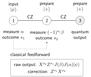
Solid edges represent CZ preparation; the dashed arrow carries a classical outcome. The first measurement uses $\alpha$ and returns $s_1$. The second uses $(-1)^{s_1}\beta$ and returns $s_2$. Removing or tracking the output frame $X^{s_2}Z^{s_1}$ leaves the logical state $J(\beta)J(\alpha)|\psi\rangle$.

A two-wire entangling kernel uses inputs $1,2$, outputs $3,4$, and edges

$$E=\bigl\{ \{1,3\},\{2,4\},\{3,4\} \bigr\}.$$

Measuring both inputs in the X basis gives four equiprobable branches. The logical target is

$$CZ_{34}(H\otimes H),$$

and the output frame is

$$\left(X_3^{s_1}Z_3^{s_2}\right) \otimes \left(Z_4^{s_1}X_4^{s_2}\right).$$

Thus the reusable ideal kernels are a $J(\alpha)$ step, a multistep wire or rotation, and a two-wire CZ pattern. They specify logical maps and frames, not a graph-generation protocol or hardware schedule.

Universality and physical costs

Arbitrary equatorial angles supply $J(\alpha)=HR_z(-\alpha)$, and the two-wire kernel supplies CZ. Concatenating these operations gives universal ideal qubit computation. An arbitrary graph need not have this capability: universality concerns a suitable family of resource graphs and allowed measurements. Universal gate sets distinguishes exact continuous controls from a finite set with approximation error.

For an ideal pattern, count supplied inputs, prepared plus-state vertices, CZ edges, measurements and classical outcomes separately. Measurement rounds also differ from the feedforward steps between them: one measurement round has no earlier result to wait for; two adaptively linked rounds have one such dependency stage. Commuting CZ gates still compete for shared hardware, so their number alone does not determine preparation depth or execution time.

Loss, noisy preparation and nonideal measurement change the implemented channel. Photonic qubits discusses physical resource generation; fault-tolerant gates and the threshold theorem address encoded noisy computation. The qubit formulas here do not describe finite-squeezing errors in continuous-variable computation or prove security of blind and delegated computation.

Worked example: one measurement and a random byproduct

Supply $|+\rangle$ at vertex 1, prepare $|+\rangle$ at vertex 2 and entangle them with CZ. Measure vertex 1 at $\alpha=\pi/3$. The two exact branch maps are

$$K_s=\frac{e^{-i\pi/6}}{\sqrt2}X^sJ(\pi/3), \qquad p_0=p_1=\frac12.$$

After the $X^s$ correction, both branches have target state

$$|\phi\rangle=J(\pi/3)|+\rangle =\frac{\sqrt3}{2}|0\rangle+\frac{i}{2}|1\rangle.$$

Forgetting the result without correcting instead gives

$$\frac12|\phi\rangle\langle\phi| +\frac12X|\phi\rangle\langle\phi|X=\frac{I}{2}.$$

Its purity and squared overlap with $|\phi\rangle$ are both $1/2$; its trace distance from the pure target is $1/2$. The mixture $I/2$ is specific to this input. For input $|0\rangle$, the corrected target is $|+\rangle$ up to phase, and both raw branches already have that same ray because $X|+\rangle=|+\rangle$. Such a favorable input does not make the uncorrected channel correct for arbitrary inputs.

The pattern uses one supplied input, one prepared plus state, one CZ, one measurement and one recorded bit. It has one measurement round and no adaptive measurement dependency; the output still carries the known byproduct unless it is corrected.

Worked example: why the second angle must adapt

On the three-vertex path, supply $|+\rangle$, choose $\alpha=\pi/3$, $\beta=\pi/4$, and measure at $\beta'=(-1)^{s_1}\pi/4$ in the second round. Each of the four outcomes has probability $1/4$. Applying the inverse output frame $Z^{s_1}X^{s_2}$ gives $J(\pi/4)J(\pi/3)|+\rangle$ in every branch, up to a branch phase. Its amplitudes are

$$a_0=\frac{\sqrt3e^{i\pi/8}+ie^{-i\pi/8}}{2\sqrt2} \simeq0.701057+0.560986i,$$ $$a_1=\frac{\sqrt3e^{i\pi/8}-ie^{-i\pi/8}}{2\sqrt2} \simeq0.430459-0.092296i.$$

Now keep the second measurement fixed at $+\pi/4$ while retaining the same final frame correction. Branches with $s_1=0$ are unchanged. For $s_1=1$, the corrected output has squared overlap $5/8$ with the intended target; averaging over all four branches gives $13/16$. This coherent error cannot be repaired by merely flipping the second classical outcome.

The ideal pattern uses three vertices, two CZ edges, two measurements and two bits. There are two measurement rounds with one feedforward stage between them. If both algorithmic angles were zero, both measurements would be in X and could occur in the same round, with the final frame processed afterward.

Common pitfalls

Normalizing too early hides probabilities. Keep the branch scalar until $K_{\mathbf s}^\dagger K_{\mathbf s}$ has been calculated. Agreement of corrected normalized states alone does not check normalization of the full channel.

A frame is information about an unperformed correction. It must be used in a later gate, measurement basis or reported result. Ignoring it generally changes the logical output.

Basis sign and outcome relabeling are different. Adding $\pi$ swaps the two outcomes, whereas changing a generic angle to its negative changes the physical basis. Pauli angles are special cases.

Exercises

Translate an Equatorial-Basis Convention

An author uses

$$|\pm_\alpha\rangle_{\mathrm{alt}} = \frac{|0\rangle\pm e^{-i\alpha}|1\rangle}{\sqrt2}.$$

Translate the one-bit kernel into this convention and identify the logical $J$ operation.

Solution

The alternative state at angle $\alpha$ is the page’s state at angle $-\alpha$:

$$|\pm_\alpha\rangle_{\mathrm{alt}} =|\pm_{-\alpha}\rangle.$$

Substitute $-\alpha$ into the exact one-bit identity:

$$(\langle s_\alpha|_{\mathrm{alt}}\otimes I) CZ (|\psi\rangle\otimes|+\rangle) = \frac{e^{i\alpha/2}}{\sqrt2} X^sJ(-\alpha)|\psi\rangle.$$

Thus the normalized corrected action is $J(-\alpha)=HR_z(\alpha)$, up to global phase. The sign change records a relabeling of the basis parameter, not a different physical projector or channel.

Parallelize a Three-Node Pauli Wire

Set both algorithmic angles on a three-vertex path to zero. Determine the four branch probabilities, logical action, output frame, and physical measurement depth.

Solution

Here $J(0)=H$, so the corrected logical action is

$$J(0)J(0)=H^2=I.$$

The three-path identity gives probability $1/4$ for each $(s_1,s_2)$ and raw output

$$X_3^{s_2}Z_3^{s_1}|\psi\rangle.$$

The second commanded angle is $(-1)^{s_1}0=0$, independent of $s_1$. Both physical measurements are therefore X measurements and may occupy one measurement layer. The logical flow order $1\prec2\prec3$ remains useful for interpreting and processing the output frame; physical parallelism does not erase that dependency structure.

Consume an Incoming Pauli Frame

A logical qubit arrives with frame $X^xZ^z$. Derive the command that implements algorithmic equatorial angle $\alpha$, and determine which dependency may be converted into a reported-bit flip.

Solution

Commuting the incoming frame into the measurement command gives

$$M^\theta X^xZ^z =M^{(-1)^x\theta+z\pi}.$$

Equivalently, the physical command that realizes the desired logical angle is

$$\theta=(-1)^x\alpha+z\pi \pmod{2\pi}.$$

Adding $\pi$ exchanges $|+_\theta\rangle$ and $|-_\theta\rangle$, so one may omit the $z\pi$ shift and report $s=r\mathbin{\oplus}z$, where $r$ is the raw detector bit. By contrast, changing $\alpha$ to $-\alpha$ generally rotates to a different basis. The $x$ dependency cannot be replaced by a bit flip except at special Pauli angles or under a declared symmetry.

Derive a Two-Wire Entangling Pattern

Let $V=\{1,2,3,4\}$, $I=\{1,2\}$, $O=\{3,4\}$, and

$$E=\bigl\{ \{1,3\},\{2,4\},\{3,4\} \bigr\}.$$

Measure inputs 1 and 2 in the X basis. Find the branch probabilities, corrected target, and raw output frame.

Solution

Each input-to-output edge implements a one-bit step, while $CZ_{34}$ commutes with the two input projections. The two independent X-basis outcomes therefore give four branches with

$$p(s_1,s_2)=\frac14.$$

The logical one-bit steps supply $H\otimes H$, and the output edge supplies the entangler, so the corrected target is

$$CZ_{34}(H\otimes H).$$

Flow choices $f(1)=3$ and $f(2)=4$ give the direct $X_3^{s_1}$ and $X_4^{s_2}$ corrections. Because output 4 is the other neighbor of $f(1)=3$, outcome $s_1$ also contributes $Z_4^{s_1}$. Similarly, $s_2$ contributes $Z_3^{s_2}$. The raw frame is therefore

$$\left(X_3^{s_1}Z_3^{s_2}\right) \otimes \left(Z_4^{s_1}X_4^{s_2}\right).$$

Verify Flow on a Five-Vertex Path

For the path $1$–$2$–$3$–$4$–$5$ with input 1, output 5, and algorithmic angles $\alpha_1,\ldots,\alpha_4$, verify $f(i)=i+1$ and derive the commanded angles, output frame, and generic number of adaptive measurement rounds.

Solution

For each measured $i$, vertex $f(i)=i+1$ is adjacent to $i$ and later in the order

$$1\prec2\prec3\prec4\prec5.$$

The only other neighbor of $f(i)$, when it exists, is $i+2$, which is also later than $i$. All flow conditions hold. Propagating the $X$ and $Z$ components from earlier outcomes gives

$$\theta_1=\alpha_1, \qquad \theta_2=(-1)^{s_1}\alpha_2,$$ $$\theta_3=(-1)^{s_2}\alpha_3+s_1\pi, \qquad \theta_4=(-1)^{s_3}\alpha_4+s_2\pi.$$

The remaining output frame is

$$X_5^{s_4}Z_5^{s_3}.$$

For generic non-Pauli angles, each measurement command can depend on the preceding record, so there are four measurement rounds and three sequential feedforward stages. Special Pauli angles can permit signal shifting, but they do not change the generic count.

Read Out a Framed Logical Qubit

A logical output carries frame $X^xZ^z$ and is to be measured at algorithmic equatorial angle $\alpha$. Give two equivalent correct readout procedures and reject the tempting generic shortcut.

Solution

One may send the fully repaired command

$$\theta=(-1)^x\alpha+z\pi \pmod{2\pi}$$

to the measurement device and use its returned bit directly. Equivalently, command

$$\theta=(-1)^x\alpha$$

and convert the raw result $r$ to the logical result $s=r\mathbin{\oplus}z$. The alternatives are equivalent because the omitted $z\pi$ term only swaps the two basis labels.

There is no generic procedure that commands $\alpha$ and compensates $x$ with a bit flip: the $X$ frame changes $\alpha$ to $-\alpha$, which is generally a different equatorial basis.

Count Accepted Resource States

Every preparation attempt consumes 25 vertices, 32 entanglers, and 23 measurements. Attempts are independent, each resource is accepted with probability $0.8$, and 1,000 accepted outputs are required. Find the expected number and variance of attempts, its standard deviation, and the expected resource totals.

Solution

For the number $N$ of Bernoulli attempts required to obtain $r=1000$ acceptances with $p=0.8$, the negative-binomial moments are

$$\mathbb E[N] =\frac{r}{p} =1250,$$ $$\operatorname{Var}(N) =\frac{r(1-p)}{p^2} =312.5, \qquad \sigma_N =17.67766953.$$

Every attempt spends all listed resources, including rejected attempts. Multiplying the per-attempt costs by $\mathbb E[N]$ gives

$$\mathbb E[\text{vertices}] =31{,}250,$$ $$\mathbb E[\text{entanglers}] =40{,}000, \qquad \mathbb E[\text{measurements}] =28{,}750.$$

These are expected costs, not a fixed-run guarantee. A time per attempt, parallelism model, and controller model were not supplied, so throughput and wall-clock latency are N/A.

Measure a four-vertex wire in parallel

For the path $1$–$2$–$3$–$4$, use input vertex 1, output vertex 4 and zero algorithmic angles. Show how to measure vertices 1, 2 and 3 in X simultaneously, process their raw bits $r_1,r_2,r_3$, and correct the output for an arbitrary input. What happens to input $|+\rangle$?

Solution

The sequential flow prescription has angles $0,0,s_1\pi$. The last $\pi$ shift changes only the label, so all physical measurements can instead be X measurements in one round. Set

$$s_1=r_1,\qquad s_2=r_2,\qquad s_3=r_3\oplus r_1.$$

The logical operation is $J(0)^3=H$. Every branch has probability $1/8$, and the raw output is

$$X^{r_3\oplus r_1}Z^{r_2}H|\psi\rangle$$

up to a global phase. Apply the inverse frame $Z^{r_2}X^{r_3\oplus r_1}$, or keep the two frame bits for later use. For input $|+\rangle$, the corrected output is $|0\rangle$.

This pattern uses one supplied input, three prepared plus states, three CZ edges and three measurements. The classical processing includes one XOR and produces two final frame bits. One simultaneous measurement round eliminates intermediate adaptive waiting, but the output correction still depends on the recorded results.

References

• H. J. Briegel, D. E. Browne, W. Dür, R. Raussendorf, and M. Van den Nest, “Measurement-based quantum computation,” Nature Physics 5, 19–26 (2009), doi:10.1038/nphys1157.
• D. E. Browne, E. Kashefi, M. Mhalla, and S. Perdrix, “Generalized flow and determinism in measurement-based quantum computation,” New Journal of Physics 9, 250 (2007), doi:10.1088/1367-2630/9/8/250.
• V. Danos and E. Kashefi, “Determinism in the one-way model,” Physical Review A 74, 052310 (2006), doi:10.1103/PhysRevA.74.052310.
• V. Danos, E. Kashefi, and P. Panangaden, “The measurement calculus,” Journal of the ACM 54(2), article 8 (2007), doi:10.1145/1219092.1219096.
• M. Hein, J. Eisert, and H. J. Briegel, “Multiparty entanglement in graph states,” Physical Review A 69, 062311 (2004), doi:10.1103/PhysRevA.69.062311.
• M. Mhalla and S. Perdrix, “Finding optimal flows efficiently,” ICALP 2008, Part I, Lecture Notes in Computer Science 5125, 857–868 (2008), doi:10.1007/978-3-540-70575-8_70.
• M. A. Nielsen, “Cluster-state quantum computation,” Reports on Mathematical Physics 57, 147–161 (2006), doi:10.1016/S0034-4877(06)80014-5.
• M. A. Nielsen and C. M. Dawson, “Fault-tolerant quantum computation with cluster states,” Physical Review A 71, 042323 (2005), doi:10.1103/PhysRevA.71.042323.
• R. Raussendorf and H. J. Briegel, “A One-Way Quantum Computer,” Physical Review Letters 86, 5188–5191 (2001), doi:10.1103/PhysRevLett.86.5188.
• R. Raussendorf, D. E. Browne, and H. J. Briegel, “Measurement-based quantum computation on cluster states,” Physical Review A 68, 022312 (2003), doi:10.1103/PhysRevA.68.022312.
• R. Raussendorf, J. Harrington, and K. Goyal, “Topological fault-tolerance in cluster state quantum computation,” New Journal of Physics 9, 199 (2007), doi:10.1088/1367-2630/9/6/199.
• M. Van den Nest, A. Miyake, W. Dür, and H. J. Briegel, “Universal resources for measurement-based quantum computation,” Physical Review Letters 97, 150504 (2006), doi:10.1103/PhysRevLett.97.150504.