Graph States

A graph state is a multipartite qubit state specified by a simple undirected graph. Vertices are qubits, edges prescribe entangling controlled-$Z$ operations, and the resulting state is characterized by a set of commuting Pauli products supported on vertices and their neighbors.

Graph states are important because they turn complicated multipartite entanglement into combinatorial data. They include cluster states used in measurement-based quantum computing, give compact examples of stabilizer states, and provide useful test cases for entanglement witnesses and quantum error correction.

Helpful background. Composite operators makes the omitted identity factors precise; Pauli matrices supplies the commutation rules used in the stabilizers.

Graphs and Qubits

Let

$$G=(V,E)$$

be a simple undirected graph with vertex set

$$V=\{1,2,\ldots,n\}.$$

Each vertex labels one qubit, so the Hilbert space is

$$\mathcal H_G = \bigotimes_{v\in V}\mathbb C^2.$$

The neighborhood of a vertex $v$ is

$$N(v) = \{u\in V:\{u,v\}\in E\}.$$

Thus the graph records which qubits are directly connected in the state-preparation circuit. It is not, by itself, a physical lattice unless a particular implementation supplies one.

Controlled-Z Construction

Start with every qubit in

$$\lvert+\rangle = \frac{1}{\sqrt2} \bigl( \lvert0\rangle+\lvert1\rangle \bigr), \qquad \lvert+\rangle^{\otimes n}.$$

For each edge $\{i,j\}\in E$, apply the controlled-$Z$ gate

$$CZ_{ij} = \operatorname{diag}(1,1,1,-1)$$

on qubits $i$ and $j$ in the computational basis. The graph state is

$$\lvert G\rangle = \prod_{\{i,j\}\in E} CZ_{ij} \lvert+\rangle^{\otimes n}.$$

All controlled-$Z$ gates are diagonal in the computational basis, so they commute. The product therefore does not depend on the order of the edges.

Equivalently,

$$\lvert G\rangle = \frac{1}{2^{n/2}} \sum_{x\in\{0,1\}^{n}} (-1)^{ \sum_{\{i,j\}\in E}x_i x_j } \lvert x_1x_2\cdots x_n\rangle.$$

The exponent is interpreted modulo $2$: every edge whose two endpoint bits are both $1$ contributes a minus sign.

First Examples

If $E$ is empty, then

$$\lvert G\rangle = \lvert+\rangle^{\otimes n},$$

so the state is fully product.

For a graph with two vertices and one edge,

$$\lvert G\rangle = CZ\lvert++\rangle = \frac{1}{2} \bigl( \lvert00\rangle + \lvert01\rangle + \lvert10\rangle - \lvert11\rangle \bigr).$$

This is an entangled two-qubit state. It is locally unitarily equivalent to a Bell state. For example, applying a Hadamard gate to the second qubit gives

$$(I\otimes H)\lvert G\rangle = \frac{1}{\sqrt2} \bigl( \lvert00\rangle+\lvert11\rangle \bigr) = \lvert\Phi^+\rangle.$$

For a three-qubit path graph

$$1-2-3,$$

the graph state is a linear three-qubit cluster state. For a star graph with one center connected to all other vertices, the graph state is locally Clifford equivalent to a GHZ state: apply a Hadamard to every leaf, leaving the center unchanged. The center generator becomes $X^{\otimes n}$ and each leaf generator becomes $Z_{\rm center}Z_{\rm leaf}$.

These equivalences are useful, but they do not mean the graph is irrelevant. Different graphs organize correlations, measurements, and code constructions in different ways.

Stabilizer Description Preview

Graph states have a compact Pauli-eigenvalue description. For each vertex $v$, define

$$K_v = X_v \prod_{u\in N(v)} Z_u,$$

where $X_v$ acts as the Pauli $X$ on qubit $v$, and $Z_u$ acts as the Pauli $Z$ on qubit $u$.

The graph state is the unique simultaneous $+1$ eigenstate of all these operators:

$$K_v\lvert G\rangle = \lvert G\rangle, \qquad v\in V.$$

The reason is simple. The product state $\lvert+\rangle^{\otimes n}$ is stabilized by every $X_v$:

$$X_v\lvert+\rangle^{\otimes n} = \lvert+\rangle^{\otimes n}.$$

Conjugating $X_v$ by the controlled-$Z$ gates incident on $v$ gives

$$\left( \prod_{\{i,j\}\in E} CZ_{ij} \right) X_v \left( \prod_{\{i,j\}\in E} CZ_{ij} \right) = X_v\prod_{u\in N(v)}Z_u.$$

Thus the simple $X_v$ stabilizers of $\lvert+\rangle^{\otimes n}$ become the graph-state stabilizers $K_v$.

The operators $K_v$ commute with each other. If two vertices are not adjacent, the corresponding Pauli factors do not conflict. If two vertices are adjacent, each stabilizer has one $X$ where the other has one $Z$, giving two anticommutations in the product and hence an overall commutation.

Linear Cluster Example

For the path graph $1-2-3$, the neighborhoods are

$$N(1)=\{2\}, \qquad N(2)=\{1,3\}, \qquad N(3)=\{2\}.$$

The stabilizer generators are

$$K_1=X_1Z_2, \qquad K_2=Z_1X_2Z_3, \qquad K_3=Z_2X_3.$$

These three commuting observables specify the three-qubit graph state as their common $+1$ eigenstate. Notice that each stabilizer is local in the graph-theoretic sense: it acts on a vertex and its neighbors.

For a longer one-dimensional chain, the interior generators have the form

$$K_j = Z_{j-1}X_jZ_{j+1}.$$

This pattern is the algebraic signature of a one-dimensional cluster state.

Entanglement from Graph Connectivity

Disconnected graphs give product states across connected components. If

$$G=G_1\sqcup G_2,$$

with no edge connecting the two components, then

$$\lvert G\rangle = \lvert G_1\rangle\otimes \lvert G_2\rangle$$

up to the ordering convention for tensor factors.

Connected graph states are entangled across every nontrivial bipartition of the vertices. More quantitatively, for a bipartition $A\vert\bar A$, the Schmidt rank of a graph state is determined by the adjacency matrix connecting the two sides:

$$\operatorname{SR}_{A\vert\bar A}(\lvert G\rangle) = 2^{r_A}, \qquad r_A = \operatorname{rank}_{\mathbb F_2} \Gamma_{A,\bar A}.$$

Here $\Gamma_{A,\bar A}$ is the submatrix of the graph adjacency matrix with rows in $A$ and columns in $\bar A$, and the rank is over the two-element field $\mathbb F_2$. This formula is one reason graph states are analytically tractable: some entanglement data can be read from binary linear algebra.

The formula should not be mistaken for a full multipartite classification. Graph states are a structured family, not the space of all multipartite states.

The nonzero reduced-state eigenvalues are all $2^{-r_A}$, so the entropy in bits is also $S(\rho_A)=r_A$. This is a binary matrix rank, not a count of crossing edges and not generally the rank over the real numbers (Hein, Eisert, and Briegel).

For example, let $A=\{1,2\}$ and $B=\{3,4\}$. Two separate edges $1-3$ and $2-4$ give $\Gamma_{A,B}=I_2$, rank two, and two bits of entropy. Connecting every vertex of $A$ to every vertex of $B$ gives $\Gamma_{A,B}=\begin{pmatrix}1&1\\1&1\end{pmatrix}$, rank one, and only one bit. More crossing edges need not mean more entanglement across a specified cut.

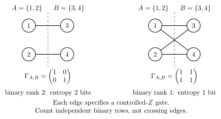
Two independent crossing edges give two bits of entanglement across $A:B$. Four crossing edges with identical adjacency rows give only one bit. The dashed line marks the chosen partition; the edge count alone does not determine the Schmidt rank.

Cluster states and measurements

A cluster state is a graph state on a lattice such as a line or square grid. In measurement-based quantum computation, the graph is combined with designated input/output qubits, adaptive single-qubit measurement bases, and outcome-dependent corrections. A graph state alone is not yet a computational protocol; for example, a one-dimensional chain is not a universal resource for arbitrary quantum computation under single-qubit measurements.

A simple state-level rule illustrates the role of outcomes. Measuring vertex $v$ in $Z$ with outcome bit $m$ removes that vertex and its incident edges. The state on the remaining vertices is

$$\left(\prod_{u\in N(v)}Z_u^m\right)|G-v\rangle,$$

with probability $1/2$ for either outcome. Thus the remaining graph is known up to local $Z$ corrections. Forgetting the outcome instead produces a mixture of the two branches. Photonic qubits discusses how destructive measurements and photon loss affect such preparations.

Reading an edge correctly

An edge specifies a controlled-$Z$ in this preparation, not necessarily an interaction that remains switched on. Nor does it promise entanglement in the two-qubit marginal of its endpoints: in the three-vertex path, all pair marginals are separable because the state is locally equivalent to GHZ. The graph describes a global state, and local Clifford changes can give different graphs for equivalent entanglement patterns.

References

• M. Hein, J. Eisert, and H. J. Briegel, “Multiparty entanglement in graph states”, Physical Review A 69, 062311 (2004).
• M. Hein, W. Dür, J. Eisert, R. Raussendorf, M. Van den Nest, and H.-J. Briegel, “Entanglement in graph states and its applications”, in Quantum Computers, Algorithms and Chaos, IOS Press (2006), pp. 115–218.
• R. Raussendorf and H. J. Briegel, “A one-way quantum computer”, Physical Review Letters 86, 5188–5191 (2001).
• M. Van den Nest, J. Dehaene, and B. De Moor, “Graphical description of the action of local Clifford transformations on graph states”, Physical Review A 69, 022316 (2004).

Exercises

1. Show that all controlled-$Z$ gates in the graph-state construction commute.

Solution

Each controlled-$Z$ gate is diagonal in the computational basis. Diagonal matrices commute with each other, even when they act on overlapping qubits. Therefore the product

$$\prod_{\{i,j\}\in E}CZ_{ij}$$

is independent of the order chosen for the edges.

2. Compute the two-qubit graph state for one edge and verify that applying $I\otimes H$ gives $\lvert\Phi^+\rangle$.

Solution

Starting from

$$\lvert++\rangle = \frac12 \bigl( \lvert00\rangle+\lvert01\rangle+\lvert10\rangle+\lvert11\rangle \bigr),$$

the controlled-$Z$ gate flips the sign only on $\lvert11\rangle$:

$$\lvert G\rangle = \frac12 \bigl( \lvert00\rangle+\lvert01\rangle+\lvert10\rangle-\lvert11\rangle \bigr).$$

Using

$$H\lvert0\rangle = \frac{\lvert0\rangle+\lvert1\rangle}{\sqrt2}, \qquad H\lvert1\rangle = \frac{\lvert0\rangle-\lvert1\rangle}{\sqrt2},$$

one finds

$$(I\otimes H)\lvert G\rangle = \frac{1}{\sqrt2} \bigl( \lvert00\rangle+\lvert11\rangle \bigr).$$

3. For the path graph $1-2-3$, verify that $K_1=X_1Z_2$ and $K_2=Z_1X_2Z_3$ commute.

Solution

The only qubits where nonidentity Pauli operators from both products meet are qubits $1$ and $2$. On qubit $1$, $X_1$ anticommutes with $Z_1$. On qubit $2$, $Z_2$ anticommutes with $X_2$. These two minus signs cancel, so

$$K_1K_2 = K_2K_1.$$

4. If a graph has two disconnected components $G_1$ and $G_2$, show that the graph state factors across those components.

Solution

The initial state factors:

$$\lvert+\rangle^{\otimes n} = \lvert+\rangle_{G_1}^{\otimes \lvert V_1\rvert} \otimes \lvert+\rangle_{G_2}^{\otimes \lvert V_2\rvert}.$$

Because there are no edges between components, the controlled-$Z$ gates split into a product of gates internal to $G_1$ and gates internal to $G_2$. Hence

$$\lvert G\rangle = \lvert G_1\rangle\otimes\lvert G_2\rangle$$

up to tensor-factor ordering.

5. For a six-vertex graph cut into $A=\{1,2,3\}$ and $B=\{4,5,6\}$, let the cross-adjacency matrix be

$$\Gamma_{A,B}=\begin{pmatrix}1&1&0\\1&0&1\\0&1&1\end{pmatrix}.$$

Compute the Schmidt rank and entropy. Why would real matrix rank give the wrong answer?

Solution

Over $\mathbb F_2$, the third row is the sum of the first two, while the first two are independent. Thus $r_A=2$, Schmidt rank is $2^2=4$, and entropy is two bits. Over the reals the determinant is $-2$, so the real rank is three. Graph-state phase addition is modulo two, which is why that real rank is irrelevant here.