Time-Dependent Perturbation Theory and Transitions

A weak time-dependent interaction changes amplitudes by accumulating contributions over time. Whether those contributions reinforce or cancel depends on the energy gap, drive frequency, pulse shape, and duration. This chapter develops transition probabilities first, then explains when summing over a continuum produces an approximately constant rate.

Helpful background. Time-dependent Hamiltonians and the interaction picture explain the evolution being approximated. Small parameters and error estimates explains why weak coupling need not give a uniformly accurate long-time answer.

Enter this chapter

Begin with the interaction picture for perturbation theory, then ordered transition amplitudes and first-order transition probability. The first separates the known reference motion; the second organizes successive interactions; the third connects amplitudes to a measurement probability.

Time ordering is part of exact evolution. Truncating the Dyson expansion is the approximation. A transition is defined relative to a chosen basis: an interaction can leave energy-basis populations unchanged while changing phases that matter to another measurement.

Resonance is coherent accumulation

Let $H(t)=H_0+\lambda V(t)$, with a system prepared in an eigenstate $\lvert i\rangle$ of $H_0$. For a different final eigenstate $\lvert f\rangle$, the leading interaction-picture amplitude is

$$c_f(t)\approx-\frac{i\lambda}{\hbar} \int_{t_0}^{t}e^{i\omega_{fi}(t'-t_0)}V_{fi}(t')\,dt',$$

where $\omega_{fi}=(E_f-E_i)/\hbar$. The matrix element supplies the coupling; the phase compares the drive with the energy gap. If $V_{fi}(t)=W_{fi}e^{-i\omega t}$ during a square pulse of duration $T$, then the leading probability is

$$P_{i\to f}(T)\approx \frac{\lambda^2\lvert W_{fi}\rvert^2T^2}{\hbar^2} \operatorname{sinc}^2\left(\frac{\delta T}{2}\right), \qquad \delta=\omega_{fi}-\omega,$$

where $\operatorname{sinc}x=\sin x/x$ and its value at zero is one. Here $W_{fi}$ is one Fourier component of the drive matrix element; a real sinusoidal field generally has both positive- and negative-frequency components.

On resonance, the contributions add coherently and the leading probability grows as $T^2$. At nonzero detuning they partly cancel. Longer pulses resolve narrower frequency intervals, of order $1/T$. This finite-time line shape follows from Fourier analysis, without introducing a time operator.

The harmonic-perturbation page develops the two frequency components. Resonant driving and the weak-drive Rabi limit explain when coherent few-level dynamics must replace the growing first-order result. Monitor the total probability of leaving the initial state, not only each final channel separately.

Why a continuum can produce a rate

For a single final level, the coherent probability above is not a constant-rate law. A continuum changes the calculation: many final energies contribute, with a density of states and a coupling that must be normalized consistently.

The finite-time factor

$$K_T(\delta)=T\operatorname{sinc}^2(\delta T/2)$$

has area $2\pi$ on the whole frequency axis. It becomes taller and narrower as $T$ grows. When integrated against a smooth spectral weight, it approaches $2\pi\delta_{\mathrm D}(\delta)$, where $\delta_{\mathrm D}$ denotes the Dirac delta distribution. This is an integrated limit, not a pointwise replacement at finite time.

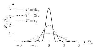
The curves show $K_T/t_*$ against $\delta t_*$ for $T=t_*,2t_*,4t_*$, using an arbitrary reference time $t_*$. Their full areas are all $2\pi$; the tails extend beyond the plotted interval. A smooth continuum averages over the narrowing peak and yields a probability approximately proportional to $T$.

The resulting golden rule requires an observation window: long enough to resolve the smooth spectral envelope, but short enough that depletion and finite-size recurrences remain negligible. Schematically,

$$\tau_{\mathrm{corr}}\ll T\ll \min(\Gamma^{-1},t_{\mathrm{rec}}).$$

A sharp threshold or structured spectral density can spoil the simple rate law. The density-of-states page explains the final-state measure and the conversion between frequency and energy delta functions. A rate is not supplied merely by dividing any finite-time probability by its duration.

Symmetry, pulse speed, and observables

Selection rules in transition rates explain why matching the frequency is insufficient: a forbidden matrix element still vanishes on resonance. For spectroscopy, light–matter transition rates connect polarization and dipole matrix elements to absorption and emission. The linear-response introduction turns the same weak-drive reasoning into a change in an observable and a susceptibility.

The chapter also compares different time limits. The sudden approximation applies when a change leaves too little time for appreciable state evolution. The adiabatic approximation follows a sufficiently separated instantaneous eigenspace during a slow change. The Landau–Zener transition shows how a sweep through a small avoided-crossing gap can connect these regimes. A slow laboratory sweep is not automatically adiabatic if the gap is very small.

Exercises

Same fluence or same amplitude? For the square-pulse formula, hold $W_{fi}$ fixed and double $T$. What happens to the resonant leading probability and the first-zero detuning? State the condition needed to trust the probability change.

Solution

The resonant probability increases by a factor of four, and the first-zero magnitude $2\pi/T$ is halved. The result assumes the total transition probability remains small. It holds at fixed drive amplitude; keeping total pulse energy fixed would instead change that amplitude.

No population transfer, but a phase change. Let $H_0=(\hbar\omega_0/2)\sigma_z$ and $V(t)=v(t)\sigma_z$. Which populations remain constant? What phase change does the perturbation add?

Solution

The $\sigma_z$ populations remain constant because the Hamiltonian stays diagonal in that basis. The added relative phase of the $+z$ and $-z$ amplitudes is $-2\lambda\int v(t)\,dt/\hbar$. This is the extra phase due to the perturbation; the reference Hamiltonian contributes its own phase. An initial superposition can therefore show changed $\sigma_x$ measurement probabilities.

Probability order. If $c_f=\lambda a_f+\lambda^2b_f+O(\lambda^3)$ for an initially empty channel, what is the next correction after $\lambda^2\lvert a_f\rvert^2$?

Solution

Squaring the amplitude gives $2\lambda^3\operatorname{Re}(a_f^*b_f)$, followed by terms of order $\lambda^4$. A symmetry may remove the cubic term, but it is not absent in a general problem. “First-order transition probability” conventionally means the probability built from the first-order amplitude.

References

• C. Cohen-Tannoudji, B. Diu, and F. Laloë, Quantum Mechanics, Vol. 2, Wiley, 1977. Time-dependent perturbations and transitions.
• J. J. Sakurai and J. Napolitano, Modern Quantum Mechanics, 3rd ed., Cambridge University Press, 2020. Transition amplitudes, selection rules, and the golden rule.
• B. Zwiebach, Quantum Physics III, MIT OpenCourseWare 8.06, Chapter 4, 2018. Finite-time transitions, harmonic driving, and rates.