Small Parameters and Error Estimates

A small parameter tells you which limit to explore; an error estimate tells you how much a particular answer may change. They are related, but they are not the same statement. This page uses an exactly solvable two-level model to distinguish a small mixing ratio, an omitted-term estimate, and a proved error bound.

Helpful background. Matrix diagonalization supplies the two-state eigenvalue calculation, and asymptotic analysis explains finite expansions and remainders.

Dimensionless mixing and a two-level example

Consider a Hermitian matrix in an orthonormal basis,

$$H=\begin{pmatrix}0&v\\v&\Delta\end{pmatrix}, \qquad \Delta>0,\qquad v\in\mathbb R.$$

The uncoupled states differ in energy by $\Delta$. The dimensionless mixing parameter is $\epsilon=v/\Delta$, not $v$ alone. The characteristic equation $E(E-\Delta)-v^2=0$ gives the lower energy

$$\begin{aligned} \frac{E_-}{\Delta} &=\frac{1-\sqrt{1+4\epsilon^2}}{2}\\ &=-\epsilon^2+\epsilon^4-2\epsilon^6+\cdots. \end{aligned}$$

Keeping the first nonzero correction gives $E_{\mathrm{pt}}=-v^2/\Delta$. It is accurate at small $\lvert\epsilon\rvert$, but becomes unreliable when the coupling is comparable with the gap. The figure shows the error growing continuously; there is no universal sharp boundary between “small” and “large.”

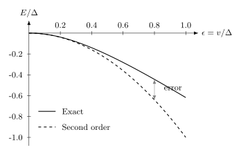
The solid curve is $E_-/\Delta$ and the dashed curve is $-\epsilon^2$. Their vertical separation is the absolute energy error in units of $\Delta$. At $\epsilon=0.1$ the error is about $9.8\times10^{-5}$; at $\epsilon=1$ it is about $0.382$.

Turn the next term into a bound when possible

The next term suggests an error of order $\Delta\epsilon^4$. In this model we can prove more. Rationalizing the square root twice gives the exact difference

$$\begin{aligned} E_--E_{\mathrm{pt}} &=\Delta\left[\epsilon^2- \frac{2\epsilon^2}{1+\sqrt{1+4\epsilon^2}}\right]\\ &=\frac{4\Delta\epsilon^4} {\left(1+\sqrt{1+4\epsilon^2}\right)^2}. \end{aligned}$$

The denominator is at least $4$, so

$$0\le E_--E_{\mathrm{pt}}\le\Delta\epsilon^4.$$

This inequality holds for all real $\epsilon$, although it becomes a loose bound at large coupling. A requested absolute accuracy $\delta E$ is therefore guaranteed if $\Delta\epsilon^4\le\delta E$. The bound comes from the displayed inequality. Merely noticing that the next coefficient is positive would not establish it for an arbitrary problem.

For this model, the power series about zero has radius of convergence $1/2$, set by complex square-root branch points. The error inequality above does not require summing that series. A finite approximation can have a useful bound even outside a series’ disk of convergence.

Many small couplings can accumulate

For a nondegenerate eigenstate, the first-order correction is a sum over other states. With an orthonormal discrete basis, its squared norm is

$$\lVert\delta n\rVert^2 =\sum_{m\ne n} \frac{\lvert V_{mn}\rvert^2} {\lvert E_n^{(0)}-E_m^{(0)}\rvert^2}.$$

Every individual ratio being small is not sufficient when there are many of them. If $M$ independent contributions each have magnitude $r$, their total correction norm is $\sqrt M\,r$. This is a necessary scale check on weak mixing, not a general convergence theorem. Continua require the corresponding normalized integrals, and operator-domain questions matter for unbounded perturbations. See first-order state corrections for the derivation and interpretation.

Specify which error matters

For an observable $Q$, an absolute error is $\lvert Q_{\mathrm{app}}-Q\rvert$. A relative error divides by $\lvert Q\rvert$ and is useful only when that reference is nonzero and physically relevant. Close to an exact zero or a tiny level splitting, a different scale may be needed.

The notation $R_N(\epsilon)=O(\epsilon^{N+1})$ is a statement about a limit: the ratio $\lvert R_N\rvert/\lvert\epsilon\rvert^{N+1}$ stays bounded sufficiently near zero, at fixed $N$. It does not give the constant or the useful parameter range. Nor does it guarantee uniformity in another variable such as time, distance, or level number. The DLMF definitions make these distinctions precise.

For example, $\sin^2(\alpha t)=(\alpha t)^2+O((\alpha t)^4)$ is useful when $\lvert\alpha t\rvert\ll1$. Small $\alpha$ at fixed $t$ is different from taking $t$ proportional to $1/\alpha$. The Rabi example shows this loss of long-time accuracy in a quantum transition.

Checks with different strengths

Check	What it establishes
A rigorous remainder inequality	A quantitative bound within its stated assumptions
A next-order calculation	An error estimate when a justified hierarchy relates that term to the remainder
A variational trial energy	An upper bound for the spectral bottom, not a two-sided error bar or a general observable bound
Conservation of norm, flux, or symmetry	A necessary consistency condition; passing it does not determine the error
Basis, grid, or time-step refinement	Sensitivity to that numerical approximation; other limits must be tested separately

For WKB, a useful local diagnostic is $\hbar\lvert p'\rvert/\lvert p\rvert^2\ll1$, where $p=\sqrt{2m(E-V)}$ in an allowed region. It fails at a simple turning point, requiring matching. It is not itself a global numerical error bar; rapidly varying higher derivatives can also require attention. For scattering, the Born-series remainder has a bound only when an appropriate operator norm is controlled; practical Born validity tests are often less conclusive.

Use the error-estimate checklist to collect the observable, regime, retained order, and independent checks in a finished calculation.

Exercises

An accuracy target. Let $\Delta=1\,\mathrm{eV}$. What sufficient restriction on $\lvert v\rvert$ guarantees an error no greater than $10^{-4}\,\mathrm{eV}$ for $E_{\mathrm{pt}}$?

Solution

The bound requires $\epsilon^4\le10^{-4}$, hence $\lvert\epsilon\rvert\le0.1$ and $\lvert v\rvert\le0.1\,\mathrm{eV}$. At the endpoint the exact error is about $9.805\times10^{-5}\,\mathrm{eV}$, slightly below the bound.

Collective mixing. There are $10^4$ orthogonal first-order contributions of magnitude $0.01$. Does inspecting each coefficient separately support weak mixing?

Solution

No. Their squared magnitudes sum to $1$, so the first-order correction has norm $1$. The correction is comparable with the normalized starting state even though every individual coefficient is small.

A suspicious next term. A first correction is $0.02$ and the second is $0.015$ in the same units. What should you conclude?

Solution

The displayed terms do not show a strong hierarchy. This may indicate an unsuitable parameter range, or an accidentally suppressed first correction. It does not by itself prove divergence. Compare with another method or establish more information about the remainder before assigning an error bar.

Choose an error scale. A calculation predicts two energies of order $1\,\mathrm{eV}$, separated by $10^{-6}\,\mathrm{eV}$. Each energy is individually known only to $10^{-4}\,\mathrm{eV}$. Is the splitting established?

Solution

No. The individual error estimates are much larger than the splitting. Correlated errors could cancel, but that cancellation needs a separate argument or a direct calculation of the difference. Good relative accuracy for each total energy is insufficient.

References

• M. V. Berry and K. E. Mount, “Semiclassical approximations in wave mechanics”, Reports on Progress in Physics 35, 315–397, 1972. Local WKB conditions and uniform approximations.
• F. W. J. Olver and R. Wong, “Definitions and Elementary Properties,” §2.1, in NIST Digital Library of Mathematical Functions, Chapter 2: Asymptotic Approximations.
• B. Zwiebach, “Non-degenerate and Degenerate Perturbation Theory”, Quantum Physics III, MIT OpenCourseWare 8.06, 2018. Spectral perturbation theory and its validity.