Variational and Bound Methods

A variational calculation guesses a family of possible states and adjusts it to lower the energy. For a self-adjoint Hamiltonian bounded below, every admissible trial state gives an energy at or above the bottom of the spectrum. This makes variational methods useful even when there is no small coupling to expand in. The important question is how much the chosen family can improve, and what a good energy tells us about the state.

Helpful background. Expectation values explain the quantity being minimized; energy eigenstates and spectral decomposition explain the bound. Small parameters and error estimates distinguish a bound from an accuracy estimate.

What the variational bound means

Write $E_0=\inf\sigma(H)$ for the bottom of the spectrum. The Rayleigh quotient of a nonzero trial state is

$$\mathcal R_H[\psi] =\frac{q_H[\psi]}{\langle\psi\vert\psi\rangle} \geq E_0,$$

where $q_H$ is the energy quadratic form. If $H\psi$ exists as a Hilbert-space vector, its numerator is the familiar $\langle\psi\rvert H\lvert\psi\rangle$. Using the form allows a larger class of finite-energy states. Its domain imposes the appropriate boundary and regularity conditions; these need not be every derivative condition in the operator domain. For example, a hard-wall trial function must vanish at the wall, whereas a Neumann kinetic-energy form does not require its trial functions to have zero derivative there.

For a discrete spectrum, the physical reason for the inequality is simple: the expectation is a probability-weighted average of eigenvalues, none below $E_0$. The variational principle proves the statement including continuous-spectrum cases. When $E_0$ is not an eigenvalue, normalizable states can approach the bound without attaining it.

An ansatz is a restricted family of trial states, such as Gaussians with adjustable widths. Let $E_{\mathcal T}$ be the infimum of the energy in that family. Then

$$E_0\leq E_{\mathcal T}\leq E[\psi_{\mathrm{found}}].$$

The last inequality holds for any admissible state found in the family, even when the optimization is incomplete. It concerns exact energy expectations. A numerical quadrature or finite-sample estimate can fluctuate below the true expectation and does not automatically preserve the bound.

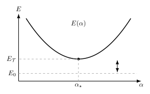
Lowering the energy within a trial family reaches $E_{\mathcal T}$ at an optimal parameter $\alpha_\star$, if the minimum is attained. The remaining separation from $E_0$ comes from the restricted family. A better optimizer cannot remove that separation; a more expressive family may.

Choose a first calculation

Start with the harmonic-oscillator estimate. One adjustable Gaussian width balances kinetic localization against potential energy, and the exact solution provides a check. Then try the helium estimate: an effective nuclear charge describes screening, while the missing electron correlation explains why the result is approximate.

The next choice is how to represent the trial state:

Representation	What you vary	Where to learn it
A chosen wavefunction shape	Widths, decay lengths, or correlation factors	Trial wavefunctions and variational parameters
A finite linear span	Coefficients of basis states	Rayleigh–Ritz method
Correlated Gaussians	Width matrices and linear coefficients	Gaussian variational methods
A many-particle trial state	Parameters whose energy is sampled statistically	Variational Monte Carlo

In a linear span the optimization becomes $Hc=ESc$, where $S$ is the overlap matrix. Accurate matrix elements and a well-conditioned independent basis matter as much as the eigensolver. Increasing the basis size gives monotone improvement only when the spaces are nested and the same Hamiltonian is evaluated accurately.

What an accurate energy does and does not imply

A one-sided bound is not a two-sided error bar. Two similar upper bounds can both be far from the true energy. Compare physically different trial families, enlarge the family systematically, and check the observable you actually want.

A small spectral gap makes energy especially insensitive to state errors. For a nondegenerate ground state separated from the rest of the spectrum by $\Delta>0$, a normalized trial state satisfies

$$1-|\langle0\vert\psi\rangle|^2 \leq \frac{E[\psi]-E_0}{\Delta}.$$

This is useful only when the energy excess and a positive gap bound are known. An energy error of $10^{-3}$ in chosen units can be excellent when the gap is $1$, and inconclusive when the gap is $10^{-4}$. Even with a large overlap, an unbounded observable such as a high position moment needs additional control of the tails.

Excited levels require extra care. Simply making a state orthogonal to an inaccurate ground-state approximation does not guarantee an upper bound to the first excited energy. The min–max principle explains the ordered Ritz bounds and their spectral assumptions. Exact symmetry restrictions can also select the lowest state in an invariant sector.

Beyond static energy minimization

Two extensions use the word “variational” differently. Variational perturbation theory introduces an adjustable reference problem and reorganizes a series; an optimized truncated series is not automatically a Rayleigh upper bound. Time-dependent variational dynamics chooses motion within a state family to approximate the Schrödinger equation, rather than continually lowering the energy.

For a calculation that gives an implausible result, common variational pitfalls explains how to distinguish an inadmissible trial state, inaccurate integration, incomplete optimization, and a family that cannot represent the required physics.

Exercises

Why normalization matters. Show that the Rayleigh quotient is unchanged by $\psi\mapsto c\psi$ for nonzero complex $c$. Why can minimizing the unnormalized numerator give a meaningless answer?

Solution

Both numerator and denominator acquire $|c|^2$, which cancels. The numerator alone can approach zero by shrinking the state whenever its energy numerator is positive; if it is negative, it can run to minus infinity by increasing the norm. Neither operation improves the state’s shape. Fix the norm or minimize the quotient.

Enlarging a family. If $\mathcal T_1\subseteq\mathcal T_2$, show that $E_0\leq E_{\mathcal T_2}\leq E_{\mathcal T_1}$. Does increasing the number of parameters always imply this ordering?

Solution

Every state available in the smaller family remains available in the larger, so the infimum cannot increase. The variational principle supplies the lower bound $E_0$. More parameters do not establish inclusion: two different functional forms may describe non-nested families. The ordering also says nothing by itself about the size of the remaining error.

A zero-variance state. An approximate state has exactly zero energy variance. Must it be the ground state?

Solution

No. When the required moments exist, zero variance implies $(H-\langle H\rangle)\psi=0$, so the state is an eigenstate. Every exact excited eigenstate also passes this test. Its energy and, when relevant, its symmetry sector identify the state.

References

• MacDonald, J. K. L. “Successive Approximations by the Rayleigh–Ritz Variation Method.” Physical Review 43, 830–833 (1933). doi:10.1103/PhysRev.43.830. Ordered variational eigenvalues and successive trial spaces.
• Nesbet, R. K. Variational Principles and Methods in Theoretical Physics and Chemistry. Cambridge University Press (2003). doi:10.1017/CBO9780511535161. Static and dynamical variational formulations.
• Reed, M., and B. Simon. Methods of Modern Mathematical Physics, IV: Analysis of Operators. Academic Press (1978). Quadratic forms, spectral bounds, and the min–max principle.