Quantum Error Correction and Fault Tolerance

Quantum error correction protects quantum information by encoding it into a larger physical system and measuring carefully chosen checks. The checks reveal information about errors while preserving the unknown logical state. Fault tolerance adds a further requirement: the operations used to protect and compute with that state must not let a few faults spread into an uncorrectable error.

This chapter connects the mathematical idea to actual computation. You will learn how a code defines logical information, how syndrome measurements and decoders guide recovery, and how logical gates, thresholds and resource requirements fit together. A good first goal is to understand why measuring a parity can reveal an error without measuring the qubit being protected.

Required background. The circuit model introduces gates, ancillas, measurement and feedforward. Noise in quantum information explains channels, correlations and leakage.

Helpful background. Quantum information carriers distinguishes physical systems from logical encodings. Pauli matrices supplies the algebra used below.

Enter this chapter

Start with why error correction is possible, then learn the Pauli group, stabilizer formalism and syndrome measurements. The three-qubit codes make those ideas concrete before codes protecting against general single-qubit errors are introduced.

From there, choose a question:

• How do small codes protect against both bit and phase errors? Compare the five-qubit, Shor and Steane codes. CSS codes explain how suitable pairs of classical codes produce quantum codes.
• How does geometry affect protection? Study the surface code, color codes and the common ideas of topological codes.
• What changes when checks are sparse or gauge variables are introduced? Quantum LDPC codes address sparse check families; subsystem codes separate protected logical information from gauge degrees of freedom.
• Can one oscillator carry a logical qubit? Begin with bosonic codes, then compare cat, binomial and GKP encodings. Their physical redundancy occupies oscillator states, with finite energy and control costs.
• How do measurement records become useful computation? Decoders infer a correction or logical frame. Fault-tolerant gates, magic-state distillation and lattice surgery develop logical operations and their additional resources.
• When does protection improve as the system grows? Read the threshold theorem, logical benchmarking and resource estimation together: they answer mathematical, experimental and architectural questions, respectively.

For practical calculations, stabilizer simulation supplies computational tools. Error-correction case studies examines specific demonstrations, and the fault-tolerant computing frontier discusses developing directions.

Reveal an error without revealing the logical state

Encode $\alpha|0\rangle+\beta|1\rangle$ into

$|\psi_L\rangle=\alpha|000\rangle+\beta|111\rangle.$

This is not three independent copies of the input: it is one joint state in a two-dimensional subspace. Assume for this example that at most one physical $X$ error occurs and that all checks and recovery operations are perfect. The commuting checks $Z_1Z_2$ and $Z_2Z_3$ have eigenvalue $+1$ on both code basis states. Their results therefore reveal parity, not whether the logical state is zero or one.

Error	Check eigenvalues	Recovery
$I$	$(+1,+1)$	$I$
$X_1$	$(-1,+1)$	$X_1$
$X_2$	$(-1,-1)$	$X_2$
$X_3$	$(+1,-1)$	$X_3$

For example, $X_2$ produces $\alpha|010\rangle+\beta|101\rangle$. Both terms have check values $(-1,-1)$, so ideal parity measurement leaves their relative amplitude and phase intact. Applying $X_2$ restores the encoded state.

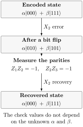
The syndrome is the same for both components of the superposition. It identifies the middle-qubit flip under the stated one-error assumption without learning $\alpha$ or $\beta$. Measuring the three individual $Z$ values would instead distinguish the components and destroy their coherence.

The general exact-correction condition of Knill and Laflamme (1997) is

$PE_a^\dagger E_bP=c_{ab}P,$

where $P$ projects onto the code and $\{E_a\}$ is the error set. The coefficients must not depend on the logical state. This condition also handles coherent combinations of correctable errors and preservation of entanglement with another system. Its derivation belongs in why error correction is possible.

The three-qubit example protects only against the specified bit flips. A single $Z_1$ changes the relative phase between $|000\rangle$ and $|111\rangle$ without changing either check. Its full Pauli distance is therefore one, not three. A general distance-$d$ quantum code corrects arbitrary errors on up to $\lfloor(d-1)/2\rfloor$ qubits in the ideal recovery setting. The fault model still matters: one correlated physical event can affect several qubits.

A syndrome is a clue, not a unique cause

The table assumes at most one error. Two flips $X_2X_3$ give the same syndrome as $X_1$, but applying the table’s recovery then leaves $X_1X_2X_3$, a logical bit flip. These errors differ logically; this ambiguity is not the same as two errors differing by a stabilizer and acting identically on the code.

With independent bit flips of probability $p<1/2$, the one-flip explanation is more probable. At $p=.08$, the probabilities of $X_1$ alone and $X_2X_3$ alone are $.067712$ and $.005888$. Given that syndrome, the table’s recovery fails with probability $.08$. Summing over all syndromes gives total logical failure $3p^2-2p^3\simeq.01818$. Correlated errors can change the best decision even though the parity algebra is unchanged.

A decoder therefore uses a noise model as well as the measured checks. Often it only needs to choose the correct logical equivalence class, not reconstruct the microscopic fault. Recovery may be a physical gate or a tracked Pauli-frame update that changes how later operations and measurements are interpreted.

Real checks are noisy. Repeated measurements help distinguish a temporary readout mistake from a persistent data error. If a raw binary check history is $(0,0,1,0,0)$, adjacent differences flag both the appearance and disappearance of the isolated wrong result. Initial and final boundary information must also be specified. Decoder throughput and the time needed for an adaptive decision can limit performance even when offline decoding works well.

Fault tolerance protects the correction process too

A code’s existence does not guarantee a safe measurement circuit. An ancilla interacts with several data qubits to measure a check; a fault on that ancilla can propagate through later gates to several data qubits. Gate ordering, verified ancillas, flags or other constructions must ensure that the allowed few faults leave a recoverable error.

Likewise, a logical gate is not automatically fault tolerant. Transversal gates constrain propagation by coupling corresponding physical qubits in different blocks, while other methods use teleportation, code deformation or gauge fixing. Stabilizer preparations, Clifford gates and Pauli measurements alone are insufficient for universal quantum computation; a suitable non-Clifford resource is also needed. Gottesman (2010) develops these connections between codes, circuits and computation.

Memory experiments test only part of that operation set. A processor also needs logical interactions, movement or routing, adaptive control and often resource-state preparation. Comparing memory lifetime with one physical constituent is useful, but it does not by itself establish a useful universal computer.

Understand scaling and practical cost

A threshold theorem states that sufficiently weak noise of a specified kind can be suppressed through a family of fault-tolerant constructions as computation grows. It depends on the allowed correlations, circuit locations, recovery and accuracy criterion. There is no architecture-independent threshold percentage. Aliferis, Gottesman and Preskill (2006) give a concrete concatenated-code analysis, including explicitly stated noise assumptions.

Numerical models also differ. A code-capacity calculation assumes perfect syndrome information; a phenomenological model adds abstract check errors; a circuit-level model includes faults during extraction gates, preparation, measurement and idling. Their threshold numbers are not interchangeable.

Finite improvement is valuable on its own. Suppose two matched sizes have $240$ and $100$ failures in one million independent trials each. Their estimated failure probabilities are $.00024$ and $.00010$, with suppression ratio $2.4$. An approximate 95% independent-binomial interval for that ratio is $[1.90,3.03]$. This supports a finite comparison under its statistical assumptions. It neither proves improvement at every larger size nor identifies break-even without a named unencoded reference. Rates per round, per complete experiment and per second also differ.

Resources include data carriers, syndrome ancillas, elapsed cycles, decoding, routing and non-Clifford state production. Discarded runs still consume resources. For a workload with failure events $F_j$, the union bound

$\Pr\!\left(\bigcup_jF_j\right)\leq\sum_j\Pr(F_j)$

allows a conservative total failure budget without independence. Each component bound must remain valid in the complete computation; omitted shared faults can invalidate the calculation. QEC protects quantum information, while mitigation usually estimates selected classical outputs. They can be combined without being interchangeable.

Exercises

1. Compare parity and individual measurements

Start with $(|000\rangle+|111\rangle)/\sqrt2$. Compare ideal measurement of the two checks with individual $Z$ measurements whose outcomes are then ignored.

Solution

Both checks are certainly $+1$, so measuring them leaves the pure state unchanged. Individual measurements distinguish $000$ from $111$ and remove the off-diagonal coherence when their results are ignored. The resulting mixture has equal populations but only fidelity $1/2$ with the original pure state. Preserving populations is insufficient for preserving a qubit.

2. Explain an ambiguous syndrome

Verify that $X_1$ and $X_2X_3$ have the same check signs. Derive the total failure probability of the table’s decoder for independent bit flips.

Solution

Each error anticommutes with $Z_1Z_2$ and commutes with $Z_2Z_3$, giving $(-1,+1)$. The decoder fails on every two-flip pattern and on the three-flip pattern, so $p_L=3p^2(1-p)+p^3=3p^2-2p^3$. This is a restricted bit-flip model with perfect checks, not a general quantum-code threshold result.

3. Interpret finite suppression

In the million-trial example, what must be matched before comparing the two sizes, and what extra comparison would establish a particular break-even claim?

Solution

Match the stored logical information, experiment duration or round count as appropriate, preparation/readout scope, decoder procedure, selection rule and failure denominator. A break-even statement additionally needs a named physical or unencoded reference protecting the same information under a specified duration and resource comparison. Two encoded sizes alone do not supply that reference or establish asymptotic scaling.

4. Allocate a total failure budget

A computation contains $10^6$ logical locations. If each location’s failure probability in the composed process is at most $10^{-9}$, what total bound follows? Does the reasoning require independent failures?

Solution

The union bound gives failure probability at most $10^6\times10^{-9}=10^{-3}$, without independence. Include preparation, readout, storage and resource-state failures in the location list or bound them separately. The statement fails if the individual bounds were measured in an isolated setting and do not apply to the composed computation.

References

• P. Aliferis, D. Gottesman, and J. Preskill, “Quantum Accuracy Threshold for Concatenated Distance-3 Codes,” Quantum Information and Computation 6, 97–165 (2006), doi:10.26421/QIC6.2-1, arXiv:quant-ph/0504218.
• D. Gottesman, “An Introduction to Quantum Error Correction and Fault-Tolerant Quantum Computation,” in Quantum Information Science and Its Contributions to Mathematics, Proceedings of Symposia in Applied Mathematics 68, 13–58 (2010), doi:10.1090/psapm/068/2762145, arXiv:0904.2557.
• E. Knill and R. Laflamme, “Theory of Quantum Error-Correcting Codes,” Physical Review A 55, 900–911 (1997), doi:10.1103/PhysRevA.55.900.