Stabilizer Simulation

A stabilizer simulator follows a quantum circuit by tracking Pauli constraints instead of every complex amplitude. For stabilizer inputs, Clifford gates and Pauli measurements, this description remains polynomial in the number of qubits. The state may still be highly entangled and have exponentially many nonzero amplitudes.

Here we connect that compression to concrete data structures, measurement sampling and error-correction calculations. The guarantee concerns a bounded number of circuit operations and efficiently evaluated classical conditions; an arbitrarily long classical computation or nonterminating loop is not made efficient by using Clifford gates.

Helpful background. Stabilizer Formalism develops the Pauli and symplectic algebra. Quantum Circuit Simulation provides a state-vector comparison, and Why Quantum Error Correction Is Possible explains syndromes and recovery.

A Bell state as two constraints

Start with two qubits in their zero states. The stabilizers are $Z_1$ and $Z_2$: the state has eigenvalue $+1$ for both. After a Hadamard on the first qubit and a CNOT from the first to the second, the generators change as follows.

After operation	First generator	Second generator
preparation	$Z_1$	$Z_2$
$H_1$	$X_1$	$Z_2$
CNOT	$X_1X_2$	$Z_1Z_2$

The final constraints specify the Bell state. They give correlations without constructing its amplitude array. Signs matter: multiplying the last two generators gives $-Y_1Y_2$, so the expectation of $Y_1Y_2$ is $-1$. The sign of a stabilizer is a physical eigenvalue condition, not the global phase of a state vector.

Why closure changes the cost

A pure stabilizer state is specified by $n$ independent commuting Pauli generators with signs, generating a group that does not contain $-I$. Aaronson and Gottesman give a standard tableau simulation algorithm. An augmented Aaronson–Gottesman-style tableau commonly stores $n$ stabilizer rows and $n$ destabilizer rows, each with $2n$ binary Pauli coordinates and phase data. Its raw binary scale is therefore

$$M_{\mathrm{tab}} = O(n^2)\ \mathrm{bits},$$

compared with

$$M_{\mathrm{sv}} = O(2^n)\ \mathrm{complex\ numbers}$$

for a generic state vector. The exact constants depend on representation, alignment, word packing, scratch space, and whether both a tableau and its inverse are retained.

For example, a raw $2n\times(2n+1)$ binary array at $n=1{,}000$ contains about four million bits, or roughly half a mebibyte before overhead. A 1,000-qubit state vector is not merely inconvenient; its $2^{1000}$ amplitudes cannot be stored by any foreseeable classical machine.

The compression works because Clifford evolution maps Pauli constraints to Pauli constraints. It does not mean that the stabilizer state’s full amplitude list is short. A graph state can have support on exponentially many basis states while its generator description remains polynomial.

Polynomial does not mean constant

The classic augmented-tableau algorithm applies a local Clifford gate by updating relevant columns and phases across the rows, giving linear work in $n$ in a straightforward layout. Pauli measurement may require row reduction and can take quadratic work. Alternative representations change these costs. An inverse tableau can make deterministic single-qubit measurements linear; graph-state representations can favor circuits whose evolving graph remains sparse; sparse or bit-packed tableaus change constants and sometimes practical scaling.

The correct performance statement therefore names the representation and operation mix. “Stabilizer circuits are efficient” is a complexity-class statement, not a benchmark result for every implementation and every output.

Which outputs remain compact?

The natural outputs are not generic amplitude arrays.

Output	Meaning	Typical cost driver
final tableau or generators	compact final stabilizer description	Clifford updates and canonicalization
one measurement trajectory	sampled outcomes with conditional state updates	number and type of Pauli measurements
many shots	repeated outcome or detector samples	analysis cost, frame propagation, output volume
Pauli expectation	$0$, $+1$, or $-1$ for a pure stabilizer state	membership and sign query
syndrome or detector stream	parity checks derived from measurements	circuit execution and parity transform
logical observable sample	encoded output bit or eigenvalue	logical definition and frame correction
Clifford action	symplectic action plus phase data	circuit compilation or tableau propagation
stabilizer-state overlap	exact structured overlap	elimination or graph operations

For a pure stabilizer state and Hermitian Pauli $P$,

$$\langle P\rangle = \begin{cases} +1, & P\in S,\\ -1, & -P\in S,\\ 0, & P\notin\pm S. \end{cases}$$

This makes Pauli observables especially convenient. A general non-Pauli observable must be decomposed into Pauli terms or handled by another method, and the number of terms may itself be large.

Sampling is efficient even when listing the full output distribution is not. A circuit can have exponentially many possible bitstrings. The simulator produces one trajectory or a requested number of shots without enumerating all outcomes.

Preparations, measurements and reset

The basic efficiently simulated operations are:

• preparation of stabilizer states such as computational-basis and graph states;
• Clifford gates, commonly generated by $H$, $S$, and CNOT;
• measurement of Hermitian Pauli observables;
• discard and reset implemented within stabilizer operations;
• classical control that selects later stabilizer operations from measurement results.

A measurement result convention must be explicit. This page uses bit $m\in\{0,1\}$ for eigenvalue

$$\lambda_m=(-1)^m.$$

Thus bit 0 means the $+1$ eigenspace and bit 1 means the $-1$ eigenspace. Some APIs expose eigenvalues directly, and others invert selected readout bits to make noiseless detector parities zero.

Reset to $\lvert0\rangle$ can be represented as a $Z$ measurement followed by an $X$ correction when the measured bit is one. The correction may be applied to the tableau or absorbed into a Pauli frame. A reset instruction must still specify whether its measurement result is retained, discarded, or available to later classical control.

The input is outside this basic family if it contains arbitrary state preparations, non-Clifford gates, or non-Pauli measurements not reducible to a Clifford basis change and Pauli measurement. A simulator may reject them, decompose them into a near-Clifford method, approximate them, or delegate to another backend. Silent replacement is not acceptable.

Discarding or forgetting a measurement result can produce a mixed state. For a uniform stabilizer-code state with $r<n$ independent generators,

$$\rho=2^{-n}\sum_{g\in S}g$$

has rank $2^{n-r}$. This is a compact mixed-state representation. Other options include retaining a purification or sampling a classical ensemble of pure stabilizer states. An arbitrary probabilistic mixture need not equal a uniform code-state projector, so do not label every such mixture by fewer generators. For example, discarding one half of a Bell pair leaves $I/2$, with no nontrivial single-qubit stabilizer; assigning it $+Z$ would incorrectly make it pure.

Choosing a representation

Generator-only tableaus

A generator-only representation stores independent stabilizers and signs. It is compact and sufficient for many Clifford updates. Determining a measurement’s deterministic sign can require solving a binary linear system or maintaining a canonical form. Repeated elimination may dominate circuits with many measurements.

Stabilizers and destabilizers

An augmented tableau adds rows dual to the stabilizer generators. These destabilizers are not additional physical constraints; they form a convenient symplectic completion. The paired structure supports efficient row operations, measurement updates, and state synthesis. The formal definitions and update rules are given in Stabilizer Formalism.

Forward and inverse tableaus

A forward Clifford tableau records how input Pauli operators transform through the circuit. An inverse tableau records the inverse action. The direction matters for queries. Pulling a measured Pauli backward through an inverse tableau can expose whether it is deterministic relative to the reference input without a full quadratic elimination.

Maintaining both directions costs memory and update work but can accelerate a measurement-heavy workload. A benchmark should state whether tableau analysis is included or amortized over many shots.

Graph state plus local Cliffords

Every pure qubit stabilizer state is local-Clifford equivalent to a graph state, as used in the simulation method of Anders and Briegel. A graph- state representation stores a graph and one local Clifford per vertex. It can be particularly effective when graph degree remains controlled. Local complementations and graph updates replace general row operations.

Graph density can grow, and a favorable representation for one circuit family may perform poorly for another. Canonicalization, graph mutation, and controlled-phase updates must be benchmarked on the target workload rather than inferred from qubit count.

Bit packing and layout

Binary Pauli coordinates naturally pack into machine words. XOR then performs many field operations at once, and population-parity instructions accelerate symplectic products. SIMD layouts can process several rows, columns, or shots in parallel.

Row-major layouts favor generator multiplication; column-oriented or transposed layouts can favor local gate updates. Some implementations keep multiple views or periodically transpose. The best layout depends on whether the workload is gate heavy, measurement heavy, or dominated by bulk Pauli frames.

Following one measurement trajectory

For one dynamic circuit shot, the simulator maintains a tableau and classical store. Each instruction performs one of four actions:

1. update tableau data under a Clifford gate;
2. classify a Pauli measurement as deterministic or random;
3. sample and apply the postmeasurement update when random;
4. write the result and execute later classically controlled operations.

The measurement branch is exact within the ideal stabilizer model. For a pure stabilizer state, a Pauli measurement outside $\pm S$ anticommutes with some stabilizer and has equiprobable outcomes. If it is fixed by the stabilizer group, the outcome is deterministic. With fewer than $n$ constraints in a mixed code state, a commuting Pauli outside $\pm S$ can also be random; the pure-state anticommutation test alone is insufficient. Which generator rows are replaced is representation dependent, but the resulting state and output distribution must not be.

As a small check, prepare $|+\rangle$ and measure $Z$ twice without an intervening operation. The first result is random; the second repeats it. The records are 00 and 11, each with probability one half. Independent random bits would incorrectly produce 01 and 10; repeating one fixed noiseless record would incorrectly remove the quantum randomness.

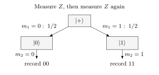
The outcomes are random individually but perfectly correlated. Their parity is always zero. A correct sampler must reproduce both the raw records and the deterministic parity.

Pauli frames and repeated samples

A Pauli frame records a Pauli correction or sampled Pauli error relative to a reference stabilizer evolution. Instead of physically applying correction $F_t$, a simulator or controller tracks it and propagates it through later Clifford gates:

$$F_t \longmapsto U_t F_t U_t^\dagger.$$

Because $U_t$ is Clifford, the frame remains Pauli. A measurement outcome flips exactly when the frame anticommutes with the measured Pauli. This often reduces correction handling to binary XOR and commutation tests.

Gidney’s Stim paper describes how a reference sample and bit-packed Pauli frames accelerate repeated sampling. Two kinds of randomness must be retained: physical Pauli faults and the circuit’s intrinsic measurement randomness. Even with no faults, the two-measurement example above must produce both allowed records. A reference record alone cannot do that.

One construction inserts appropriate random stabilizer factors into the frame at preparation and collapse steps. These factors leave the immediate reference state unchanged but produce the correct randomness in later incompatible measurements. For instance, a random $Z$ on $|0\rangle$ is initially invisible; after $H$ it becomes a random $X$ frame on $|+\rangle$, flipping the later $Z$ outcome. The complete update rule must also preserve correlations across measurements and resets.

A common-reference Pauli frame has narrower scope than a general tableau trajectory. If different measurement branches apply different non-Pauli Cliffords, the branch states need not be Pauli-related. For example, $|0\rangle$ and $H|0\rangle=|+\rangle$ cannot be related by a Pauli. Such conditional programs can still be simulated efficiently shot by shot, but need a more general branch treatment than a fixed reference plus a Pauli frame.

For a supported circuit and a correctly sampled stochastic Pauli model, frame sampling introduces no additional physical approximation. It does not make coherent rotations or leakage into Pauli errors.

Which noise can be sampled as Pauli faults?

Choose Hermitian Pauli representatives $P\in\{I,X,Y,Z\}^{\otimes n}$, with overall phases omitted. A stochastic Pauli channel has the form

$$\begin{aligned} \mathcal N(\rho)&=\sum_P p_P P\rho P,\\ p_P&\geq0,\qquad \sum_P p_P=1. \end{aligned}$$

One trajectory samples $P$ and adds it to the frame. Correlated multi-qubit faults and correlations between times can be sampled if their full joint law is available and efficiently sampled. Replacing a correlated law by independent draws changes the physical model.

Leakage and actual loss leave the qubit Pauli space. An erasure flag can be passed to a decoder, but a flag alone does not specify the conditional quantum channel. A heralded Pauli approximation must be distinguished from a model of the lost or leaked system. Amplitude damping is not a mixture of Pauli conjugations: Pauli mixtures preserve $I/2$, while damping generally does not.

Pauli twirling also changes coherent accumulation. Repeating $R_z(\theta)$ $k$ times on $|+\rangle$ gives an $X$-measurement error probability

$$p_{\mathrm{coh}}=\frac{1-\cos(k\theta)}2.$$

Replacing each rotation by an independent $Z$ error of probability $\sin^2(\theta/2)$ instead gives

$$p_{\mathrm{twirl}}=\frac{1-(\cos\theta)^k}2.$$

The two models agree for one use but generally differ after repetition. See Pauli Noise and Depolarizing Channels for the channel algebra and Noise Simulation for methods that retain more general noise.

From measurement bits to detectors

Repeated QEC circuits produce many raw ancilla measurements. A detector is a parity that has a known deterministic value in the noiseless circuit, including across its intrinsically random branches. Let $m_k$ be measurement bits. Detector $a$ is

$$d_a = b_a \oplus \bigoplus_{k\in S_a} m_k,$$

where $S_a$ identifies the included measurements and $b_a$ sets the expected reference parity. A detection event occurs when $d_a=1$.

For repeated measurement of one stabilizer check, an interior detector often compares consecutive rounds,

$$d_{r,j} = m_{r,j}\oplus m_{r-1,j}.$$

Individual gauge measurements may be random; only appropriate combinations are deterministic detectors. Boundary detectors may also include preparation or final data measurements. Their definitions depend on the experiment. A simulator should not infer them from names or geometry when an explicit parity specification is available.

Detector coordinates, times, and logical associations are metadata for a decoder. They do not change the quantum state, but mistakes in that metadata change the inferred logical performance. Noiseless simulation should verify that all declared deterministic detectors are zero for every allowed reference branch.

Decoding and logical failure

The simulator and decoder are different components.

• The simulator samples a circuit under a declared model and emits detector data plus logical-observable data reserved for scoring.
• The decoder receives only its allowed detector data and model metadata.
• The decoder predicts a correction class or logical frame.
• The evaluator compares that prediction with the withheld logical outcome.

Let $\ell\in\{0,1\}^k$ be the simulated logical-observable flips and $\widehat\ell(D)$ the decoder’s prediction from detector record $D$. A logical failure indicator is

$$f = \mathbf 1 \left[ \ell\oplus\widehat\ell(D) \neq \mathbf 0 \right].$$

Giving the decoder the sampled physical error or the true logical flip leaks ground truth and invalidates the experiment. Decoder weights may use the declared noise model, but training, tuning, and final evaluation data should be separated.

The observable definitions and correction convention must match between the simulation and decoder. A multi-bit logical record refers to jointly measurable outputs of that experiment; it does not provide simultaneous values of incompatible logical $X$ and $Z$ observables. Known preparation and final measurement conditions determine which logical flips can be scored.

Estimating logical error rates

For $N$ independent shots with $K$ failures,

$$\widehat p_L = \frac{K}{N}.$$

The uncertainty is binomial only when shots are independent and identically distributed under the declared fixed model. Shared drift, reused random contexts, adaptive stopping, or correlated batches change the statistical analysis.

When $K=0$, reporting $p_L=0$ is wrong. A one-sided upper confidence limit at confidence $1-\delta$ is

$$p_{\mathrm{upper}}=1-\delta^{1/N}.$$

At 95 percent confidence this is approximately $3/N$ for large $N$, the so-called rule of three. Resolving very small logical error rates therefore requires enormous shot counts or a validated rare-event method such as importance sampling or splitting.

Threshold studies should report physical-noise parameters, circuit and decoder, code distances, shot allocation, confidence intervals, finite-size fitting, and stopping rules. A crossing of two finite-distance curves is evidence within that protocol and noise model, not a universal hardware threshold.

Checking an error-correction calculation

Begin with the circuit without noise. Every claimed detector should vanish for every allowed branch, including random initial gauge outcomes. Then inject individual faults and compare their detector patterns with direct small-system calculations. Single-fault tests can reveal propagation or boundary mistakes; they do not establish circuit distance, which concerns combinations of faults capable of causing an undetected logical error.

Use the three-qubit repetition code as a small example. Its checks are $Z_1Z_2$ and $Z_2Z_3$. An $X_1$ fault gives syndrome $(1,0)$; an $X_2X_3$ fault gives the same syndrome. Correcting both with $X_1$ removes the first fault but leaves logical $X_1X_2X_3$ after the second. Syndrome agreement does not imply the same logical effect.

Compare a subset of circuits against an independent state-vector calculation, including conditional states and raw measurement records. Checking only detectors can miss a sampler that produces the wrong raw distribution while preserving its parities. Check sign conventions as well as commutation.

Many simulators spend time analyzing a circuit once, then sample many shots using bit-packed frames. Report both times: a good repeated-shot rate may not compensate for preparation when few shots are needed. Memory and output can also dominate; $N$ shots with $D$ detector bits contain $ND$ bits before compression, even if generating each bit is cheap. Streaming to a decoder can avoid storing the entire matrix.

Keep the circuit, detector and logical definitions, noise probabilities and correlations, simulator settings, decoder and shot count with the result. Distinguish ideal Clifford evolution, sampled Pauli noise and a Pauli approximation to another physical channel. These answer different questions.

Beyond Clifford circuits

Non-Clifford resources break basic tableau closure, but a small amount of nonstabilizer structure can sometimes be handled by decomposition. Write

$$\lvert\psi\rangle = \sum_{a=1}^{\chi} c_a\lvert\phi_a\rangle,$$

where each $\lvert\phi_a\rangle$ is a stabilizer state. Clifford gates update each term efficiently; runtime and memory depend on the number of retained terms $\chi$, overlap calculations and branching. The minimum exact term count is the stabilizer rank; a particular expansion need not achieve that minimum. For many magic resources, the retained term count can grow exponentially.

Bravyi and colleagues develop exact and approximate stabilizer decompositions. The coefficients are amplitudes, so interference between terms must be kept: a coherent sum is not a probabilistic mixture.

Quasiprobability methods decompose nonstabilizer channels into signed or complex-weighted stabilizer operations and estimate observables by weighted sampling. They can be unbiased while suffering variance that grows with the decomposition overhead, as analyzed by Pashayan, Wallman and Bartlett. “Uses stabilizer simulation” does not therefore imply polynomial total sample complexity.

Near-Clifford algorithms are valuable for circuits with limited magic and for benchmarking non-Clifford gadgets. An error and cost estimate must state whether the decomposition is exact or approximate, how coefficients are chosen, what quantity is estimated, and how variance or truncation is bounded.

One non-Clifford gate does not make every finite instance hard. It removes the general closure guarantee and introduces a resource whose scaling must be analyzed.

Common pitfalls

Dropping Pauli signs. Commuting binary coordinates are not enough. The Bell-state example distinguishes $+Y_1Y_2$ from $-Y_1Y_2$, which predict opposite deterministic outcomes.

Confusing a fast inner step with a fast full calculation. A compact tableau does not make enumeration of exponentially many outcomes cheap. Likewise, exponentially many stabilizer terms or a large sampling variance can dominate a near-Clifford calculation.

Treating zero observed failures as zero probability. State a confidence limit and the assumptions behind it. If shots were postselected, report the acceptance probability and distinguish conditional error from unconditional performance.

Exercises

1. Compare representation sizes

Estimate the raw storage of a $2n\times(2n+1)$ binary tableau at $n=1{,}000$. Compare it conceptually with a double-complex state vector.

Solution

The tableau contains

$$2{,}000\times2{,}001 = 4{,}002{,}000$$

bits, or $500{,}250$ bytes, approximately $0.477$ MiB before alignment, scratch space, and object overhead. The state vector would contain $2^{1000}$ complex amplitudes and is physically impossible to store. The comparison does not imply that every 1,000-qubit stabilizer workload is fast; circuit and sample counts still matter.

2. Classify a Bell measurement

The Bell state $\lvert\Phi^+\rangle$ is stabilized by $X_1X_2$ and $Z_1Z_2$. Is a measurement of $Z_1$ deterministic or random? What correlations remain?

Solution

$Z_1$ anticommutes with $X_1X_2$, so the measurement is random with equal probability for bits $m=0$ and $m=1$. After the measurement, the state is $\lvert00\rangle$ for $m=0$ and $\lvert11\rangle$ for $m=1$. Equivalently, the postmeasurement stabilizers can be chosen as $(-1)^m Z_1$ and $Z_1Z_2$, which imply the same eigenvalue for $Z_2$.

3. Propagate a Pauli frame

An $X$ frame error is present on the control before a CNOT from $Q_1$ to $Q_2$. The circuit then applies $H$ to $Q_2$. What is the final frame?

Solution

Under CNOT conjugation,

$$X_1 \longmapsto X_1X_2.$$

The later Hadamard maps $X_2$ to $Z_2$, so the final frame is

$$X_1Z_2.$$

No physical correction had to be inserted; the simulator updates the binary frame and flips later measurement bits when this frame anticommutes with the measured observable.

4. Construct repeated-round detectors

A noiseless check has measurement bit $1$ in every round because the prepared state is in its $-1$ eigenspace. Should the interior detector be $d_r=m_r\oplus m_{r-1}$ or simply $d_r=m_r$?

Solution

Use the parity $d_r=m_r\oplus m_{r-1}$. It is zero when the repeated result is stable, regardless of whether the reference eigenvalue is $+1$ or $-1$. Defining $d_r=m_r$ would report a detection event in every noiseless round. Boundary detectors still need explicit offsets or preparation/final data terms.

5. Score a decoder

For two logical observables, a shot has true logical-flip vector $\ell=(1,0)$ and the decoder predicts $\widehat\ell=(1,1)$. Does the shot fail under the any-logical-error rule?

Solution

The residual is

$$\ell\oplus\widehat\ell = (0,1),$$

which is nonzero. Therefore $f=1$ and the shot is a logical failure. A study may also report per-observable rates, but the aggregate rule must be declared before evaluation.

6. Bound a zero-failure result

A simulation observes no logical failures in $N=10^6$ independent shots. Give the approximate one-sided 95 percent upper bound rather than reporting zero.

Solution

Using the rule of three,

$$p_L \lesssim \frac{3}{10^6} = 3\times10^{-6}.$$

The exact binomial expression is $1-0.05^{1/10^6}$, which is very close to this value. The claim assumes a fixed sample size, independent identically distributed shots and the stated model. Repeatedly stopping when the bound looks favorable requires a sequentially valid analysis.

7. Compare coherent and twirled errors

Apply $R_z(\pi/2)$ twice to $|+\rangle$ and measure $X$. Compare the probability of the negative outcome with independently applying its Pauli-twirled channel twice.

Solution

The coherent rotations combine to $R_z(\pi)$ and take $|+\rangle$ to $|-\rangle$ up to phase, so the negative outcome has probability one. Each twirled channel applies $Z$ with probability $1/2$. The total frame is $Z$ precisely when an odd number of the two errors occurs, with probability $2(1/2)(1/2)=1/2$. Matching one-step average behavior does not preserve coherent accumulation.

8. When one reference and a Pauli frame are insufficient

An ancilla in $|+\rangle$ is measured in $Z$. If its outcome is one, apply $H$ to a second qubit initially in $|0\rangle$; otherwise do nothing. Can the second qubit’s two branch states be represented by one fixed reference state and a Pauli correction? Is the circuit still efficiently simulable?

Solution

The states are $|0\rangle$ and $|+\rangle$. Paulis take $|0\rangle$ only to $|0\rangle$ or $|1\rangle$ up to phase, so the two states are not Pauli-related. The fixed-reference frame construction is insufficient. Nevertheless every branch uses stabilizer operations; an ordinary tableau trajectory samples the ancilla and follows the selected Clifford branch in polynomial time.

9. Estimate near-Clifford growth

Suppose each of $t$ non-Clifford gadgets doubles the number of stabilizer terms in a naive exact decomposition. How many terms are present, and what does this show?

Solution

The naive expansion contains

$$N_{\mathrm{terms}}=2^t$$

stabilizer terms before cancellations or compression. This is an expansion size, not a proof that the minimum stabilizer rank equals $2^t$. Each term evolves efficiently through later Clifford gates, but the number of terms is exponential in the non-Clifford count. Stabilizer simulation remains a useful inner kernel; it does not by itself make the full near-Clifford algorithm polynomial in $t$.

10. Keep interference between stabilizer terms

Let $T=\operatorname{diag}(1,e^{i\pi/4})$. Write $T|+\rangle=a|+\rangle+b|-\rangle$ and compare its $Y$ expectation with that of a mixture weighted by $|a|^2$ and $|b|^2$.

Solution

Matching computational-basis amplitudes gives

$$\begin{aligned} a&=\frac{1+e^{i\pi/4}}2,\\ b&=\frac{1-e^{i\pi/4}}2. \end{aligned}$$

The coherent state has $\langle Y\rangle=\sin(\pi/4)=1/\sqrt2$. Each of $|+\rangle$ and $|-\rangle$ has zero $Y$ expectation, so their probabilistic mixture has zero. Replacing the coherent sum by the mixture loses the cross terms and changes the state.

11. Same syndrome, different logical effect

For the repetition-code example above, verify that $X_1$ and $X_2X_3$ have the same syndrome. If independent bit flips occur with probability $p$ on each qubit and majority correction is used, find the logical bit-flip probability for one round with perfect checks.

Solution

Both faults anticommute with $Z_1Z_2$ and commute with $Z_2Z_3$, giving $(1,0)$. Majority correction succeeds for zero or one flip and fails for two or three, so

$$p_L=3p^2(1-p)+p^3=3p^2-2p^3.$$

This small example protects against the specified bit-flip model. It is not a general quantum memory protecting against arbitrary Pauli noise.

References

• S. Aaronson and D. Gottesman, “Improved simulation of stabilizer circuits,” Physical Review A 70, 052328 (2004), doi:10.1103/PhysRevA.70.052328.
• S. Anders and H. J. Briegel, “Fast simulation of stabilizer circuits using a graph-state representation,” Physical Review A 73, 022334 (2006), doi:10.1103/PhysRevA.73.022334.
• S. Bravyi, D. Browne, P. Calpin, E. Campbell, D. Gosset, and M. Howard, “Simulation of quantum circuits by low-rank stabilizer decompositions,” Quantum 3, 181 (2019), doi:10.22331/q-2019-09-02-181.
• C. Gidney, “Stim: a fast stabilizer circuit simulator,” Quantum 5, 497 (2021), doi:10.22331/q-2021-07-06-497.
• H. Pashayan, J. J. Wallman, and S. D. Bartlett, “Estimating outcome probabilities of quantum circuits using quasiprobabilities,” Physical Review Letters 115, 070501 (2015), doi:10.1103/PhysRevLett.115.070501.