Tensor-Network Simulation

Tensor-network simulation evaluates a quantum circuit by factoring its state or its requested output into smaller arrays. It can save enormous amounts of memory when those arrays remain small. The difficulty depends on the circuit, the qubit ordering, and the output: one amplitude, an expectation value, and the full state can require very different calculations.

This page develops two approaches: evolving a matrix product state (MPS) through the gates, and contracting a network for the chosen output in an order that need not follow circuit time. Exact contraction preserves the circuit’s answer; truncating a bond introduces a state approximation whose physical meaning must be established.

Helpful background. Quantum circuit simulation defines output tasks and qubit indexing. Tensor networks introduces tensor indices and contractions, and singular value decomposition explains the factorization used to compress a bond.

Circuit amplitudes as tensor contractions

Consider an ideal circuit $U_C=U_L\cdots U_1$ acting on $\lvert0^n\rangle$. Its output amplitude is

$$A_C(x)=\langle x\rvert U_C\lvert0^n\rangle.$$

Insert computational-basis resolutions of the identity between gates. Each gate becomes an array of matrix elements, and each internal wire carries a summed basis index. For a two-qubit gate,

$$G^{a'b'}_{ab}=\langle a'b'\rvert G\lvert ab\rangle.$$

The lower indices connect to earlier gates and the upper indices to later ones. Fixing every output bit gives a scalar amplitude. Leaving some output indices open gives an array of amplitudes. The network is simply the original matrix multiplication written as smaller sums; its conversion introduces no approximation.

For example, $H$ on the first qubit followed by CNOT prepares a Bell state. The intermediate index $a$ gives

$$A(x_1x_2)=\sum_{a=0}^1 \delta_{x_1,a}\delta_{x_2,a}H_{a0}.$$

Only $00$ and $11$ have nonzero amplitudes, both $1/\sqrt2$. This little calculation already illustrates contraction: sum the shared index while preserving the uncontracted output labels.

The output changes the network

The following table assumes a pure input and an ideal unitary circuit.

Requested output	Construction	Result
One amplitude	Fix all output bits	Complex scalar
Amplitude batch	Leave $k$ output bits open	$2^k$ complex values
One probability	Square the amplitude magnitude	$p(x)$
Marginal	Join ket and bra; sum unwanted outputs	$p(x_S)$
Expectation	Insert $O$ between ket and bra	$\langle O\rangle$
Reduced state	Leave subsystem ket and bra legs open	$\rho_S$

A marginal is a sum of probabilities,

$$p(x_S)=\sum_{x_{\bar S}}|A_C(x_S,x_{\bar S})|^2,$$

not the squared magnitude of a sum of amplitudes. The doubled ket–bra network implements this distinction. Gates outside a measured observable’s backward causal cone can cancel with their adjoints, often making a local expectation much cheaper than the full state.

An explicitly requested dense output still has to be produced: a $k$-qubit reduced density matrix has $4^k$ entries. A compact network representation does not remove that output cost. It can, however, stream entries rather than keep the entire dense output in memory.

Evolving a matrix product state

An open-boundary MPS writes a coefficient as a product of matrices,

$$\Psi_{s_1\cdots s_n}=A^{[1]s_1}\cdots A^{[n]s_n}.$$

The first and last factors are a row and a column, so the product is a scalar. The bond after site $j$ has a stored dimension $\chi_j$. The physical Schmidt rank across that cut is at most $\chi_j$; equality requires a minimal representation with zero-weight directions removed. A bound $\chi_j\leq\chi$ gives dense storage $O(nq\chi^2)$ for local dimension $q$.

Vidal’s circuit simulation method exploits this structure. The MPS introduction develops canonical forms and their relation to Schmidt decompositions in more detail.

A two-site gate update

Bring the MPS into mixed canonical form with its center on the two updated sites. The left and right block states are then orthonormal. Contract the two site tensors with the gate:

$$\Theta^{s't'}_{\alpha\beta} =\sum_{s,t,\gamma}G^{s't'}_{st} A^{[j]s}_{\alpha\gamma}A^{[j+1]t}_{\gamma\beta}.$$

Reshape $\Theta$ into a matrix with row $(\alpha,s')$ and column $(t',\beta)$, factor it by SVD, and distribute the factors back to the sites. Keeping all nonzero singular values is exact up to numerical roundoff. Keeping fewer compresses the state. The orthonormal block bases are essential: only then are these singular values the physical Schmidt coefficients and their discarded squared sum a probability weight. An arbitrary gauge can make a numerically small tensor entry physically important.

For comparable bond sizes, the dense SVD costs $O(q^3\chi^3)$. This is a useful scaling law only while the required $\chi$ stays modest. A gate crossing a cut with operator Schmidt rank $r_G$ obeys

$$\chi'_j\leq r_G\chi_j,\qquad r_G\leq q^2.$$

Here the $\chi$ symbols denote the physical ranks before and after the gate. They are also bounded by the dimensions of the two sides. A two-qubit gate can multiply rank by as much as four when the boundary qubits are already entangled with other qubits; acting on a two-qubit product input can create rank at most two. Repeated layers can require exponentially growing bonds.

The same state, two different qubit orders

Prepare three independent Bell pairs, $(a_1,b_1)$, $(a_2,b_2)$, and $(a_3,b_3)$. A cut splitting $m$ pairs has $2^m$ equally weighted Schmidt coefficients: each split pair supplies an independent binary label.

Putting each pair next to its partner gives the bond ranks

$$(2,1,2,1,2).$$

Putting all $a$ qubits before all $b$ qubits gives

$$(2,4,8,4,2).$$

The physical state did not change. The second ordering simply asks an MPS bond to carry more independent correlations. For $m$ pairs the corresponding largest ranks are $2$ and $2^m$.

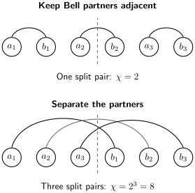
Curved lines join the partners of each Bell pair; they are not MPS bonds. The dashed central cut splits one pair in the upper ordering and all three in the lower ordering. Its exact Schmidt rank is therefore $2$ or $8$.

Nonlocal gates can be applied using swaps, changing the MPS order, or an operator network. Such transformations may increase intermediate bond sizes even if the final state is simple. Choosing an order is therefore part of choosing an efficient representation, not a change to the hardware circuit. The circuit examples studied by Zhou, Stoudenmire, and Waintal illustrate how entanglement growth limits this approach.

What discarded weight does tell you

For a normalized state with Schmidt coefficients $s_a$ in decreasing order, discarding terms beyond rank $r$ removes weight

$$\epsilon=\sum_{a>r}s_a^2.$$

If $\epsilon<1$, renormalizing the retained state gives squared-overlap fidelity $F=1-\epsilon$ and trace distance $D=\sqrt\epsilon$ from that pre-truncation state. These are one-step statements. Schollwöck explains why canonical MPS forms make such truncations physically meaningful.

There is also a useful conservative cumulative bound. Suppose an initially exact pure state undergoes the same unitary gates as the target, with normalized Schmidt truncations after selected gates. If the actual discarded weights are $\epsilon_1,\ldots,\epsilon_m$, then

$$D_{\mathrm{final}}\leq \min\left(1,\sum_{j=1}^m\sqrt{\epsilon_j}\right).$$

Unitary evolution preserves trace distance; the triangle inequality adds at most $\sqrt{\epsilon_j}$ at each truncation. Thus the total-variation distance of any final measurement distributions is at most this bound, and the error of a Hermitian observable is at most $2\lVert O\rVert D_{\mathrm{final}}$. The bound can be loose, but it is a bound; neither the sum nor the product of local infidelities is generally the exact final infidelity. Conditioning on a selected measurement outcome needs a separate analysis because normalization can amplify errors.

Entropy $S\leq\log\chi$ gives a necessary rank constraint, not a complete error estimate. Examine the Schmidt tail at the required tolerance, increase the bond cap, and compare the actual observable or distribution of interest.

Choosing a contraction order

Instead of evolving a state through time, construct the network for the requested output and contract tensors in any convenient order. Associativity preserves the exact result, but intermediate arrays can have very different sizes.

For an ordinary network in which each internal index joins two tensors, let $I$ and $J$ be their index sets and $K=I\cap J$. Contracting all shared indices produces

$$C_{(I\cup J)\setminus K}=\sum_K A_I B_J.$$

With index dimensions $d_e$, the dense multiply-add count and output size are approximately

$$W(A,B)\sim\prod_{e\in I\cup J}d_e,$$ $$|C|=\prod_{e\in(I\cup J)\setminus K}d_e.$$

A shared label that also occurs on other tensors is a hyperedge: it must remain until every required factor has been included. Summing it too early changes the calculation. Copy tensors can convert such a description to ordinary pairwise edges.

A small example of a large cost difference

Let $A$, $B$, and $C$ have shapes $2\times20$, $20\times3$, and $3\times40$. Computing $(AB)C$ uses

$$2\cdot20\cdot3+2\cdot3\cdot40=360$$

multiply-add pairs. Computing $A(BC)$ uses

$$20\cdot3\cdot40+2\cdot20\cdot40=4000.$$

The intermediate $AB$ contains 6 entries; $BC$ contains 800. Both produce the same 80-entry output. Larger networks magnify these differences.

For binary indices, define the memory width of a chosen path by $w_{\mathrm{mem}}=\log_2(\max_T|T|)$. Its largest intermediate alone needs $b2^{w_{\mathrm{mem}}}$ bytes at $b$ bytes per element. Total live memory also includes inputs, workspaces, cached tensors, and concurrent tasks.

Markov and Shi relate circuit contraction to graph treewidth: a circuit with $T$ gates and underlying graph treewidth $d$ can be simulated in $T^{O(1)}\exp[O(d)]$ time in their bounded-size gate setting. This is a structural result, not a guarantee that a practical search immediately finds the best contraction. Low depth alone does not guarantee small width on an arbitrary connectivity graph.

Greedy search, graph partitioning, and subtree optimization trade search time against later contraction cost; Gray and Kourtis describe a combined search approach. First simplify exactly where possible: fuse adjacent one-qubit gates, absorb fixed inputs, and cancel adjoint pairs outside causal cones. Diagonal and sparse gates may be much cheaper than the dense estimates above. For repeated outputs, reuse common intermediate tensors. Include the initial search cost when deciding whether that reuse is worthwhile.

Slicing indices without losing interference

Fixing a set of internal indices $S$ produces smaller contractions $Z_s$:

$$Z=\sum_{s\in\Omega_S}Z_s,\qquad |\Omega_S|=\prod_{e\in S}d_e.$$

Complete summation is algebraically exact, and different slices can run independently. Slicing an index reduces an intermediate only if that index would occur in it; arbitrary slices need not reduce the largest tensor. Repeated work can increase total cost, and running many slices concurrently can restore the memory pressure that individual slices avoided.

If $Z$ is an amplitude, add the complex slice amplitudes before taking its squared magnitude. For the circuit $HH\lvert0\rangle=\lvert0\rangle$, the amplitude of output 1 has two contributions,

$$Z_0=\tfrac12,\qquad Z_1=-\tfrac12.$$

Their sum is zero. Adding $|Z_0|^2+|Z_1|^2=1/2$ would destroy the destructive interference. A sliced index is an algebraic summation variable, not a measurement outcome.

Omitting selected slices is generally an approximation. Randomly sampled, properly weighted slices can instead define an unbiased estimator of the amplitude, with sampling uncertainty. Squaring such an estimator does not give an unbiased probability estimator automatically. Near cancellation, even complete summation may need more precision; absolute error is more informative than relative error near a zero.

Sampling and mid-circuit measurements

A normalized MPS supports direct sequential sampling using

$$p(s_j\mid s_{<j})=\frac{p(s_{\leq j})}{p(s_{<j})}.$$

Compute the two conditional probabilities, draw the next bit, update the remaining conditional state, and continue. Only positive-probability prefixes are visited, so a zero-probability branch must never be normalized. No Markov-chain equilibration is required. Sampling is exact for the represented MPS distribution, including any state approximation made earlier; this does not make it exact for the original untruncated circuit. Ferris and Vidal develop direct sampling for unitary tensor networks.

General contraction methods can also obtain conditionals from doubled networks, but one tractable amplitude does not guarantee cheap sampling: the required marginals may be harder. Caching shared prefixes or contracting several output legs together can save repeated work.

For a projective mid-circuit measurement, compute $p(m)=\langle\psi\rvert P_m\lvert\psi\rangle$, sample $m$, and evolve $P_m\lvert\psi\rangle/\sqrt{p(m)}$ through the branch selected by that record. Keeping a trajectory avoids explicitly storing every possible branch; it does not make the conditional contractions inexpensive. A discarded measurement result generally produces a mixed state, so it cannot be replaced by one arbitrary pure branch. Noise simulation develops channels, ensembles of trajectories, and density-operator networks.

Choosing and checking a calculation

Task or structure	Useful starting point	Main limitation
Local gates, modest Schmidt ranks	MPS evolution	Rank growth and ordering
A few amplitudes	Fixed-output contraction	Intermediate size
Many samples from one compact state	Reuse final MPS	Truncation error
A local expectation	Causal-cone contraction	Remaining environment
Stabilizer input and Clifford gates	Stabilizer simulation	Restricted operations

Compare small instances with a state-vector calculation, including asymmetric states that reveal reversed qubit indices. Compare alternate contraction orders and complete sliced sums. For approximate calculations, vary the bond cap and truncation threshold and inspect the requested output itself. Convergence of one expectation need not imply convergence of the full state.

The distinctions are simple but consequential: changing contraction order, exact factorization, and complete slicing change cost without changing the algebra; bond truncation and approximate environments change the answer; floating-point arithmetic adds numerical error to either calculation.

State the circuit, output, numerical precision, and approximation when describing a result. For performance comparisons, separate path-search time from contraction and sampling time and measure memory as well as operation counts. A higher-FLOP path can run faster if its matrix operations use the hardware more efficiently. Failure of one ordering or bond cap establishes the limit of that calculation, not the impossibility of every classical simulation method.

Exercises

1. Contract a Bell amplitude

The circuit prepares $\lvert00\rangle$, applies $H$ to qubit 1, and then CNOT with qubit 1 as control. Express the amplitude for output $x_1x_2$ as an index contraction and evaluate it.

Solution

Let $a$ be the basis index between $H$ and CNOT. Then

$$A(x_1x_2) =\sum_{a=0}^{1} \langle x_1x_2\rvert \mathrm{CNOT} \lvert a0\rangle \times\langle a\rvert H\lvert0\rangle.$$

CNOT maps $\lvert a0\rangle$ to $\lvert aa\rangle$, so the first factor is $\delta_{x_1,a}\delta_{x_2,a}$. Since both $\langle0\rvert H\lvert0\rangle$ and $\langle1\rvert H\lvert0\rangle$ equal $1/\sqrt2$,

$$\begin{aligned} A(00)&=A(11)=\frac{1}{\sqrt2},\\ A(01)&=A(10)=0. \end{aligned}$$

The joined index $a$ is precisely the contracted wire segment.

2. Estimate a pairwise contraction

Tensor $A_{ijk}$ has dimensions $(2,4,8)$ and tensor $B_{k\ell m}$ has dimensions $(8,3,5)$. Estimate the output size and dense multiply-add count for contracting over $k$.

Solution

The output $C_{ij\ell m}$ has

$$2\times4\times3\times5 = 120$$

elements. Each output sums over eight values of $k$, so the rough dense work is

$$2\times4\times8\times3\times5 = 960$$

multiply-add pairs. This local estimate does not include index permutation, allocation, or the effect on later intermediates.

3. Bound Schmidt-rank growth

An MPS has Schmidt rank $\chi=64$ across a cut. A two-qubit gate crossing that cut has operator Schmidt rank $r_G=2$. What upper bound follows for the exact post-gate rank? Does the rank have to reach the bound?

Solution

The operator-Schmidt expansion writes the gate as a sum of two product operators across the cut. Acting on a state of Schmidt rank 64 therefore gives rank at most

$$\chi' \leq r_G\chi = 128.$$

The actual rank may be smaller because terms can be linearly dependent or have zero weight for the particular state. The bound controls worst-case growth; it does not predict the Schmidt spectrum.

4. Interpret discarded weight

A normalized two-site update has squared Schmidt coefficients $0.70$, $0.20$, $0.08$, and $0.02$. If only two values are kept, find the discarded weight and the one-step fidelity after renormalization.

Solution

The discarded weight is

$$\epsilon_{\mathrm{disc}} = 0.08+0.02 = 0.10.$$

The normalized retained state has one-step fidelity

$$F_{\mathrm{local}} = 1-\epsilon_{\mathrm{disc}} = 0.90.$$

This does not say that ten such truncations produce final fidelity $(0.90)^{10}$ or $1-10(0.10)$. Later gates and truncations act on changed states, so a global claim needs a separate analysis.

5. Sum sliced amplitudes

For the circuit $HH\lvert0\rangle$, slice the intermediate basis index and calculate the amplitude and probability of output 1. What happens if the two slice probabilities are added instead?

Solution

The contributions are

$$H_{10}H_{00}=\tfrac12,\qquad H_{11}H_{10}=-\tfrac12.$$

Their sum is zero, so output 1 has probability zero. Adding their squared magnitudes gives $1/2$, which incorrectly removes interference. That result would describe an unread projective measurement between the Hadamards, not the original unitary circuit.

6. Choose an output strategy

You need $2^{12}$ amplitudes that share all output bits except a selected 12-qubit subset. Why might leaving those output legs open be better than running $2^{12}$ independent scalar contractions?

Solution

One contraction with 12 open binary legs can reuse every intermediate that is independent of those outputs and return a tensor with $2^{12}$ entries. Scalar repetition may redo that shared work. The open-leg plan is not automatically better: its intermediates may be larger, and the $2^{12}$-entry output must still be stored. Compare complete contraction trees and measured resource costs for both plans.

7. Sample a GHZ MPS

For

$$\lvert\mathrm{GHZ}_n\rangle = \frac{ \lvert0^n\rangle + \lvert1^n\rangle }{ \sqrt2 },$$

what are the left-to-right conditional probabilities?

Solution

The first bit is uniform:

$$p(s_1=0) = p(s_1=1) = \frac12.$$

After drawing $s_1$, every later bit is deterministic:

$$p(s_j=s_1\mid s_1,\ldots,s_{j-1}) = 1$$

for $j>1$. Direct MPS sampling therefore returns only $0^n$ and $1^n$, each with probability one half, without a Markov chain.

8. Turn local truncations into an error bound

An ideal unitary circuit is simulated with two normalized Schmidt truncations, each discarding weight $10^{-4}$. Bound the final trace distance, the error in any measurement distribution, and the expectation error of a Pauli observable. Is the final infidelity necessarily $2\times10^{-4}$?

Solution

Each truncation changes the represented pure state by trace distance $0.01$. Unitary invariance and the triangle inequality give $D\leq0.02$. Measurement cannot increase trace distance, so total-variation distance is at most $0.02$. A Pauli operator has norm one, giving expectation error at most $0.04$. For pure states, $1-F=D^2\leq4\times10^{-4}$. None of these inequalities asserts an exact accumulated error; the discarded directions can combine in different ways.

9. Why the canonical environment matters

Represent a two-qubit state by coefficient matrix $\Psi=LC$, where

$$\begin{aligned} L&=\operatorname{diag}(100,1),\\ C&=\operatorname{diag}(0.008,0.6). \end{aligned}$$

What state is represented? If the smaller singular value of $C$ is discarded and the physical state is renormalized, what fidelity remains? Compare this with the best physical rank-one approximation.

Solution

$\Psi=\operatorname{diag}(0.8,0.6)$ represents the normalized state $0.8\lvert00\rangle+0.6\lvert11\rangle$. An SVD of $C$ alone keeps its $0.6$ entry, yielding $\lvert11\rangle$ after physical normalization, with fidelity $0.36$. The misleading relative discarded squared weight in $C$ is

$$\frac{0.008^2}{0.008^2+0.6^2}\simeq1.78\times10^{-4}.$$

The physical Schmidt values are instead $0.8$ and $0.6$. Keeping the larger one yields $\lvert00\rangle$ with fidelity $0.64$. The nonorthonormal environment $L$ changes the physical metric. Canonicalization absorbs this metric before applying a physical truncation criterion.

10. Count the pairs crossing each cut

For the three-Bell-pair state in the figure, derive all five Schmidt ranks in the two orderings. If the central rank in the second ordering is truncated to two, what is the largest possible fidelity?

Solution

The adjacent-pair order splits $1,0,1,0,1$ pairs, giving ranks $(2,1,2,1,2)$. The separated-partner order splits $1,2,3,2,1$ pairs, giving $(2,4,8,4,2)$. At its central cut all eight squared Schmidt coefficients are $1/8$. Retaining two preserves weight $2/8=1/4$, the optimal rank-two fidelity at that cut. A small bond cap is highly inaccurate in this order, even though the other order represents the same state exactly with maximum bond two.

References

• A. J. Ferris and G. Vidal, “Perfect sampling with unitary tensor networks,” Physical Review B 85, 165146 (2012), doi:10.1103/PhysRevB.85.165146.
• J. Gray and S. Kourtis, “Hyper-optimized tensor network contraction,” Quantum 5, 410 (2021), doi:10.22331/q-2021-03-15-410.
• I. L. Markov and Y. Shi, “Simulating quantum computation by contracting tensor networks,” SIAM Journal on Computing 38, 963–981 (2008), doi:10.1137/050644756.
• U. Schollwöck, “The density-matrix renormalization group in the age of matrix product states,” Annals of Physics 326, 96–192 (2011), doi:10.1016/j.aop.2010.09.012.
• G. Vidal, “Efficient classical simulation of slightly entangled quantum computations,” Physical Review Letters 91, 147902 (2003), doi:10.1103/PhysRevLett.91.147902.
• Y. Zhou, E. M. Stoudenmire, and X. Waintal, “What limits the simulation of quantum computers?” Physical Review X 10, 041038 (2020), doi:10.1103/PhysRevX.10.041038.