Noise Simulation

Noise simulation predicts how an imperfect quantum process changes states and measurement outcomes. A density matrix follows the averaged state directly; stochastic trajectories follow randomly selected pure-state branches and recover that average over many runs. Both can represent the same model, but they spend memory and computation differently.

The model and the numerical method answer separate questions. Accurately solving an independent-error model does not make it describe a device with slow drift or correlated faults. This page explains how to propagate noisy circuits, preserve their measurements and correlations, and distinguish sampling uncertainty from numerical and model error.

Helpful background. Quantum circuit simulation introduces state evolution and measurement branches. Noise in quantum information describes the physical mechanisms; Kraus representations explains completely positive maps and their operator sums.

Channels acting on a circuit

For a Markovian circuit model, an ideal gate $\mathcal U_k$ and its associated noise might act as

$$\rho_{k+1}=\mathcal E_k\bigl(\mathcal U_k(\rho_k)\bigr).$$

This explicitly places the noise after the gate. Reversing their order generally changes the answer. For example, amplitude damping leaves $\lvert0\rangle$ unchanged. An $X$ gate after damping therefore gives $\lvert1\rangle$, while damping after $X$ relaxes part of that population back to $\lvert0\rangle$.

Use the implemented circuit and its timing: routing adds gates, idles expose qubits to relaxation, and simultaneous operations may introduce crosstalk. During a finite pulse, Hamiltonian and dissipative evolution generally act together. A fitted channel after each gate can be a useful phenomenological model; it need not equal the microscopic simultaneous evolution. Common noise models explains parameter conventions and their physical limits.

Density matrices and Kraus operators

For a trace-preserving channel,

$$\rho'=\sum_\alpha K_\alpha\rho K_\alpha^\dagger, \qquad \sum_\alpha K_\alpha^\dagger K_\alpha=I.$$

This averages every branch directly. An $n$-qubit density matrix contains $4^n$ complex entries, compared with $2^n$ for a pure state vector. It gives expectations without trajectory sampling error, although model parameters, floating-point arithmetic, and any numerical integration remain sources of uncertainty or error. Apply small local Kraus operators directly to the density array when possible.

With column-stacking vectorization,

$$\operatorname{vec}(A\rho B) =(B^{\mathsf T}\otimes A)\operatorname{vec}(\rho).$$

Thus the channel matrix is

$$\mathsf S_{\mathcal E}=\sum_\alpha K_\alpha^*\otimes K_\alpha.$$

It acts on $\operatorname{vec}(\rho)$, but contains $d^4$ entries for Hilbert-space dimension $d$. Constructing it explicitly can be far more expensive than applying the Kraus terms. Complex conjugation and vectorization order matter: an incorrect convention can preserve every array dimension while changing the physics.

Simulating a pure-state trajectory

For a normalized input $\lvert\psi\rangle$, calculate

$$p_\alpha=\lVert K_\alpha\lvert\psi\rangle\rVert^2.$$

Draw a branch with these probabilities and, only for $p_\alpha>0$, set

$$\lvert\psi_\alpha\rangle =\frac{K_\alpha\lvert\psi\rangle}{\sqrt{p_\alpha}}.$$

The branch probabilities generally depend on the current state. For amplitude damping of strength $\gamma$, a jump from $a\lvert0\rangle+b\lvert1\rangle$ occurs with probability $\gamma|b|^2$, not simply $\gamma$. The no-jump branch also changes the relative amplitudes.

The weighted branch projectors satisfy

$$\sum_\alpha p_\alpha \lvert\psi_\alpha\rangle\langle\psi_\alpha\rvert =\mathcal E(\lvert\psi\rangle\langle\psi\rvert).$$

Repeating this sampling through a memoryless circuit therefore reproduces its density evolution on average. One trajectory stores only a state vector, but many trajectories may be needed. A mixed initial state must also be sampled from a correctly weighted pure-state ensemble or represented by a purification; choosing one eigenvector discards part of the preparation.

The Monte Carlo wave-function methods of Dalibard, Castin, and Mølmer, reviewed by Plenio and Knight, provide the continuous-time counterpart of this idea. Johansson, Nation, and Nori describe numerical implementations in QuTiP; the current Monte Carlo guide also discusses mixed-state initial ensembles and trajectory averages.

What is sampled: branches or measurement outcomes?

Suppose the desired answer is $\langle O\rangle$. A trajectory can contribute its conditional expectation $X_r=\langle\psi_r\rvert O\lvert\psi_r\rangle$. There is no need to draw an additional terminal measurement outcome merely to estimate this mean. For independent, identically distributed trajectories at fixed model parameters,

$$\widehat\mu=\frac1N\sum_{r=1}^N X_r, \qquad \widehat{\operatorname{SE}}=\frac{s_X}{\sqrt N}.$$

If instead the goal is a realistic measurement record, sample the final outcome as well. Its variance includes quantum measurement noise. By the law of total variance, averaging conditional expectations removes that extra conditional sampling variance. A fixed-$N$ standard-error formula also needs qualification when stopping adaptively or when trajectories share a random context.

Equivalent channels can have different trajectory variance

Complete dephasing can be written in either form

$$\mathcal D(\rho)=\tfrac12(\rho+Z\rho Z) =P_0\rho P_0+P_1\rho P_1,$$

where $P_j=\lvert j\rangle\langle j\rvert$. Starting from $\lvert+\rangle$, the first representation produces $\lvert+\rangle$ and $\lvert-\rangle$ with equal probabilities. Their conditional $X$ expectations are $+1$ and $-1$, so the estimator variance is one.

The second representation produces $\lvert0\rangle$ and $\lvert1\rangle$. Each has conditional $X$ expectation zero, so this estimator has zero variance. Both averaged states are $I/2$. An actual terminal $X$ measurement nevertheless has outcomes $\pm1$ with equal probabilities in both descriptions. Changing numerical trajectories cannot remove physical measurement randomness.

If the branches describe a monitored environment, their meaning is fixed by that monitoring scheme. If they are only a computational representation, a different unraveling can improve efficiency without changing the averaged channel.

Measurement records and feedback

For a terminal measurement with effects $M_x$ and a classical assignment response $R(y\mid x)$,

$$p(y)=\sum_xR(y\mid x)\operatorname{Tr}(M_x\rho).$$

This model assumes that the effects and response describe the relevant states and context. Readout can depend on leaked levels, neighbors, or past operations. Backaction after a truly terminal measurement need not be modeled when only its outcome statistics are requested.

Mid-circuit measurements are different: their quantum instruments determine the state used by later gates. If $\mathcal I_x$ is the underlying instrument and only the noisy reported value $y$ is available, the reported branch is

$$\mathcal J_y(\rho)=\sum_xR(y\mid x)\mathcal I_x(\rho).$$

Its trace is the probability of $y$, and division by that trace gives the conditional state. Feedforward must use $y$. Sampling $x$ and then $y$ is an equivalent trajectory implementation when these latent branches are part of the chosen model; using $x$ to control a gate that sees only $y$ would give the simulated controller information the experiment lacks.

Reset may be a replacement channel, dissipative preparation, or measurement and feedback; these have different errors and timing. SPAM errors develops preparation and measurement models, and mid-circuit measurement explains the quantum–classical control sequence.

Continuous-time evolution and physical numerical steps

A time-local Lindblad model with nonnegative rates has generator

$$\dot\rho=-\frac{i}{\hbar}[H,\rho] +\sum_j\gamma_j\mathcal D[L_j](\rho),$$ $$\mathcal D[L](\rho)=L\rho L^\dagger -\tfrac12\{L^\dagger L,\rho\}.$$

Here $L_j$ is dimensionless and $\gamma_j$ has units of inverse time; alternatively absorb $\sqrt{\gamma_j}$ into the jump operator, but do not include the rate twice. Lindblad and Gorini, Kossakowski, and Sudarshan established the semigroup generators. Breuer and Petruccione discuss the physical approximations behind these descriptions. A time-local equation by itself does not establish memorylessness; see Markovian and non-Markovian noise.

For quantum jumps, the unnormalized no-jump state evolves with

$$H_{\mathrm{eff}}=H-\frac{i\hbar}{2} \sum_j\gamma_jL_j^\dagger L_j.$$

Over a short interval, the jump probability is $p_j=\gamma_j\Delta t\langle L_j^\dagger L_j\rangle+O(\Delta t^2)$. Small-step schemes must control multiple-jump errors; waiting-time methods use the survival norm to locate the next event.

Density ODE solvers and exponential-action methods offer another route. An accurate ODE method need not preserve positivity at a finite step. Conversely, a composition of exact Hamiltonian and dissipative substeps can be completely positive while still having splitting error because the generators do not commute. Refine time steps and compare the actual observable, not just trace and Hermiticity. Solving Lindblad equations and quantum-jump simulation give the detailed algorithms.

Correlations must persist across the right time interval

Consider $N$ repeated phase rotations $R_z(\delta)$ of an initial $\lvert+\rangle$. Let each individual offset have zero-mean Gaussian distribution with variance $\sigma^2$. Two models with the same single-step channel give different repeated evolution:

$$\begin{aligned} C_{\mathrm{static}}(N)&=e^{-N^2\sigma^2/2},\\ C_{\mathrm{ind}}(N)&=e^{-N\sigma^2/2}. \end{aligned}$$

Here $C=\langle X\rangle$. In the quasistatic model, one offset is drawn per run and the accumulated phase is $N\delta$. With independent offsets, the phase is a sum with variance $N\sigma^2$. Averaging its complex phase gives these Gaussian characteristic functions.

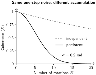
The same single-step noise does not determine a whole sequence. For $\sigma=0.2$ radians per rotation, a persistent offset gives $C(10)\simeq0.135$, whereas independent offsets give $C(10)\simeq0.819$. The curves are calculated from the displayed models.

For even $N$, an ideal sign reversal halfway through cancels the quasistatic phase exactly. Independently drawn offsets still have total variance $N\sigma^2$. Echo is therefore a useful test of the correlation assumption, not just another gate-count measurement. Draw one offset per correlation block, or a full path from the specified stochastic process; drawing fresh noise at every gate silently changes the model.

An environment that is kept or reset

An explicit system–environment calculation retains their joint state. Tracing out the environment at the end is harmless for system observables; discarding it and replacing it during the calculation generally destroys correlations that affect later evolution. Fresh independent ancillas give a memoryless collision construction. Reusing a correlated ancilla can give revivals that repeated copies of the one-step reduced channel cannot reproduce.

A process tensor describes how a sequence of interventions affects later outcomes, including temporal correlations. Pollock and colleagues develop this multitime description. Compressing an influence functional or a process tensor along time can help when its structure permits; a short two-point bath correlation alone does not guarantee a small temporal bond or justify every memory cutoff. Vary the cutoff, time resolution, and temporal bond and check the requested output.

Methods for larger or structured systems

Structure	Useful representation	Main limitation
Small general system	Density matrix	$4^n$ storage
A few means, moderate width	Pure-state trajectories	State size and variance
Stabilizer inputs, Clifford gates, Pauli faults	Tableau or Pauli frames	Restricted dynamics
Modest spatial correlations	MPO or purified tensors	Bond growth
Classical drift	State plus latent process	Correct correlation law
Quantum memory	Joint environment or process tensor	Environment or temporal size

A Pauli simulator is exact for its stated stochastic Pauli model, but twirling a coherent error changes that model. Equal one-gate average infidelity need not give equal long-sequence behavior; see stabilizer simulation.

An MPO compresses operator-space correlations rather than pure-state entanglement alone. Truncating it can break positivity. A factorization $\rho=XX^\dagger$ preserves positivity of the represented state even when $X$ is compressed, as in the locally purified approach of Werner and colleagues. It still needs trace normalization and convergence in spatial and purification dimensions. Positivity of one approximate output does not prove that the numerical procedure implements a linear completely positive channel on every input.

Explicit leakage requires extra levels, their gates, readout response, and return paths. With $n$ local $q$-level systems, density storage is $q^{2n}$. A classical leakage flag is a useful approximation only when the discarded coherences and return dynamics are irrelevant to the calculation. Leakage and crosstalk explains that physical choice. Postselected results must include their acceptance probability; a normalized accepted state does not describe rejected runs.

Parameter uncertainty and numerical uncertainty

Let $\theta$ denote uncertain model parameters and $X$ a trajectory estimator. Write $\mu(\theta)=\mathbb E[X\mid\theta]$. Then

$$\operatorname{Var}(X)= \operatorname{Var}_\theta\mu(\theta) +\mathbb E_\theta\operatorname{Var}(X\mid\theta).$$

This distinguishes variation of the predicted mean across parameter values from randomness at fixed parameters. A posterior or a defined bootstrap distribution supplies weights for parameter averaging. A confidence region alone supplies a set of possibilities, not a unique probability distribution over them; scanning that region is a sensitivity analysis.

If $M$ independent parameter draws each receive $N$ independent inner trajectories, the variance of the equally weighted nested mean is

$$\operatorname{Var}(\widehat\mu) =\frac{\operatorname{Var}_\theta\mu(\theta)}{M} +\frac{\mathbb E_\theta\operatorname{Var}(X\mid\theta)}{MN}.$$

Increasing $N$ alone cannot remove the first term. Increasing $M$ improves the numerical estimate of a chosen parameter average; it does not make the underlying calibration uncertainty vanish. For an unknown parameter fixed through a device run, keep it fixed within that simulated run. Resampling it at every gate would model physical fluctuations instead.

Common random numbers can improve differences between models, but the error bar must use the paired differences, including their covariance. Track discretization, tensor truncation, numerical precision, parameter uncertainty, and trajectory uncertainty separately. More trajectories cannot repair a wrong correlation model.

Compare small instances using density evolution and trajectory averages with uncertainty. Test trace, Hermiticity, positivity, limiting channels, and complex matrix conventions. Compare predictions with circuits and operating contexts not used to fit the parameters. If halving a time step shifts a result, compare that shift with its sampling uncertainty and repeat the refinement; one small change after doubling trajectory count does not prove that sampling error is negligible. Clipping negative density eigenvalues changes the answer and must not substitute for finding the numerical problem.

Exercises

1. Estimate density-matrix memory

How much raw memory does a complex128 density matrix require for $n=15$ qubits, before scratch space and alignment?

Solution

The matrix contains

$$4^{15} = 2^{30} = 1{,}073{,}741{,}824$$

complex entries. At 16 bytes per complex128 value, this is

$$2^{30}\times16 = 2^{34}\ \mathrm{bytes} = 16\ \mathrm{GiB}.$$

A practical update may need the input, output, Kraus workspaces, and temporary permutations simultaneously, so 16 GiB is not a sufficient machine-memory budget.

2. Sample amplitude damping

For amplitude damping with

$$K_0 = \begin{pmatrix} 1&0\\ 0&\sqrt{1-\gamma} \end{pmatrix},$$ $$K_1 = \begin{pmatrix} 0&\sqrt\gamma\\ 0&0 \end{pmatrix},$$

find the trajectory probabilities for $\lvert\psi\rangle=a\lvert0\rangle+b\lvert1\rangle$.

Solution

The jump probability is

$$p_1 = \langle\psi\rvert K_1^\dagger K_1 \lvert\psi\rangle = \gamma |b|^2.$$

The no-jump probability is

$$p_0 = |a|^2 + (1-\gamma)|b|^2 = 1-\gamma|b|^2.$$

For a nonzero-probability jump, the state is physically $\lvert0\rangle$. On no jump, it is

$$\frac{ a\lvert0\rangle + \sqrt{1-\gamma}\,b\lvert1\rangle }{ \sqrt{p_0} }.$$

Averaging the two branch projectors gives the usual amplitude-damping channel.

3. Show that placement matters

Start in $\lvert0\rangle$. Compare an ideal $X$ gate followed by amplitude damping of strength $\gamma$ with amplitude damping followed by $X$.

Solution

Applying $X$ first prepares $\lvert1\rangle$. Damping then gives

$$\rho_A = \gamma \lvert0\rangle\langle0\rvert + (1-\gamma) \lvert1\rangle\langle1\rvert.$$

Damping $\lvert0\rangle$ does nothing, and the later $X$ gives

$$\rho_B = \lvert1\rangle\langle1\rvert.$$

Thus $\rho_A\neq\rho_B$ for $\gamma>0$. A channel name and probability do not define a circuit model without composition order.

4. Estimate trajectory uncertainty

A binary logical-failure estimator observes $K=240$ failures in $N=20{,}000$ independent trajectories. Estimate the rate and its standard error using the binomial plug-in variance.

Solution

The estimate is

$$\widehat p = \frac{240}{20{,}000} = 0.012.$$

The estimated standard error is

$$\widehat{\operatorname{SE}} = \sqrt{ \frac{ \widehat p(1-\widehat p) }{ N } } \approx 7.7\times10^{-4}.$$

A report should use an appropriate binomial interval rather than treating $\widehat p\pm2\,\widehat{\operatorname{SE}}$ as exact in every regime.

5. Apply a readout response

An ideal measurement gives $p(x=1)=0.3$. The readout flips $0\to1$ with probability $0.02$ and $1\to0$ with probability $0.08$. Find the reported probability $p(y=1)$.

Solution

Using the classical response,

$$p(y=1)=0.02\,p(x=0) +0.92\,p(x=1).$$

Since $p(x=0)=0.7$,

$$\begin{aligned} p(y=1)&=0.02(0.7)+0.92(0.3)\\ &=0.29. \end{aligned}$$

This postprocessing is valid only under the declared factorization between quantum evolution and classical readout confusion.

6. Compare persistent and independent offsets

For ten phase rotations with $\sigma=0.2$ radians, calculate $\langle X\rangle$ in the two Gaussian models above. What does an ideal sign reversal after the fifth rotation change?

Solution

The persistent phase has variance $10^2(0.2)^2=4$, so $C_{\mathrm{static}}=e^{-2}\simeq0.1353$. Independent increments have variance $10(0.2)^2=0.4$, so $C_{\mathrm{ind}}=e^{-0.2}\simeq0.8187$. The sign reversal changes the persistent sum to $5\delta-5\delta=0$, giving coherence one in this ideal model. In the independent model, changing signs does not change the variance of the sum, so its coherence remains $e^{-0.2}$.

7. A trace-preserving step that is not positive

Evolve $\rho=(I+X)/2$ under $H=\hbar\Omega Z/2$. One forward-Euler step gives $\rho_E=\rho-i\Delta t[H,\rho]/\hbar$. Find its eigenvalues and explain why trace and Hermiticity checks are insufficient.

Solution

Using $[Z,X]=2iY$ and $a=\Omega\Delta t$ gives

$$\rho_E=\tfrac12(I+X+aY).$$

Its eigenvalues are

$$\lambda_\pm=\frac{1\pm\sqrt{1+a^2}}{2}.$$

The smaller eigenvalue is negative for every nonzero step, although the matrix is Hermitian and trace one. The exact unitary update rotates the Bloch vector on the unit sphere; Euler moves along a tangent outside it. Decreasing the step decreases the violation but does not make this finite-step map positive. Unitary exponentiation preserves positivity for this example.

8. Reduce estimator variance without changing the channel

Apply complete dephasing to $\lvert+\rangle$ using either Kraus set $\{I/\sqrt2,Z/\sqrt2\}$ or $\{P_0,P_1\}$. Compare the variance of the conditional $X$ expectation with the variance of a sampled terminal $X$ outcome. Do the two Kraus sets describe the same monitored record?

Solution

For the first set, the states are $\lvert\pm\rangle$, so conditional expectations are $\pm1$ and their variance is one. For the second, the states are $\lvert0\rangle,\lvert1\rangle$, so both conditional expectations are zero and their variance vanishes. Both output densities are $I/2$.

Terminal $X$ outcomes have mean zero and variance one in either case. In the second representation that variance comes entirely from the final measurement. The two Kraus sets are equivalent for unmonitored system evolution, but their branch labels correspond to different environment monitoring schemes.

9. Allocate nested samples

A parameter distribution assigns equal weights to failure probabilities $p=0.01$ and $p=0.03$. For each of $M$ independent parameter draws, simulate $N=1000$ independent Bernoulli outcomes. Find the mean and variance of the overall estimated rate. What remains if only $N$ tends to infinity?

Solution

The parameter-averaged mean is $0.02$. Across parameter draws, $\operatorname{Var}(p)=0.0001$, and the average conditional variance is

$$\tfrac12[0.01(0.99)+0.03(0.97)]=0.0195.$$

Consequently,

$$\begin{aligned} \operatorname{Var}(\widehat p) &=\frac{0.0001+0.0195/1000}{M}\\ &=\frac{0.0001195}{M}. \end{aligned}$$

At fixed $M$, increasing only $N$ leaves $0.0001/M$. Increasing $M$ improves Monte Carlo integration over the assumed parameter distribution; its physical spread $\sqrt{\operatorname{Var}(p)}=0.01$ has not disappeared.

10. Keep the environment’s memory

A system starts in $\lvert+\rangle$ and an environment qubit in $\lvert0\rangle$. Apply CNOT with the system as control twice. Compare the final system state if the environment is retained with the result if it is discarded and replaced by $\lvert0\rangle$ between gates.

Solution

The first CNOT creates a Bell pair, so the reduced system state is $I/2$. Keeping the environment lets the second CNOT undo the first, restoring $\lvert+\rangle\lvert0\rangle$. Thus the system ends pure with $\langle X\rangle=1$.

Resetting the environment removes the Bell correlations and leaves $(I/2)\otimes\lvert0\rangle\langle0\rvert$. The second CNOT then leaves the reduced system $I/2$, with $\langle X\rangle=0$. A reduced state at one time does not encode the correlations needed for later memory effects.

References

• H.-P. Breuer and F. Petruccione, The Theory of Open Quantum Systems, Oxford University Press (2002), doi:10.1093/acprof:oso/9780199213900.001.0001.
• J. Dalibard, Y. Castin, and K. Mølmer, “Wave-function approach to dissipative processes in quantum optics,” Physical Review Letters 68, 580–583 (1992), doi:10.1103/PhysRevLett.68.580.
• V. Gorini, A. Kossakowski, and E. C. G. Sudarshan, “Completely positive dynamical semigroups of N-level systems,” Journal of Mathematical Physics 17, 821–825 (1976), doi:10.1063/1.522979.
• J. R. Johansson, P. D. Nation, and F. Nori, “QuTiP 2: A Python framework for the dynamics of open quantum systems,” Computer Physics Communications 184, 1234–1240 (2013), doi:10.1016/j.cpc.2012.11.019.
• G. Lindblad, “On the generators of quantum dynamical semigroups,” Communications in Mathematical Physics 48, 119–130 (1976), doi:10.1007/BF01608499.
• M. B. Plenio and P. L. Knight, “The quantum-jump approach to dissipative dynamics in quantum optics,” Reviews of Modern Physics 70, 101–144 (1998), doi:10.1103/RevModPhys.70.101.
• F. A. Pollock et al., “Non-Markovian quantum processes: Complete framework and efficient characterization,” Physical Review A 97, 012127 (2018), doi:10.1103/PhysRevA.97.012127.
• A. H. Werner et al., “Positive tensor network approach for simulating open quantum many-body systems,” Physical Review Letters 116, 237201 (2016), doi:10.1103/PhysRevLett.116.237201.