SPAM Errors

State-preparation and measurement (SPAM) errors affect the two ends of a quantum experiment. An imperfect preparation emits a different state from the target; an imperfect measurement changes outcome probabilities or the state left afterward. The observed frequencies combine both. Even infinitely many repetitions need not tell us which end caused a discrepancy.

This page explains that ambiguity, when a classical assignment matrix describes readout, and what calibration can support. The examples use finite-dimensional systems; leakage, discarded outcomes and persistent detector memory must be included when present.

Helpful background. Measurement in circuits supplies outcome probabilities and conditional states. Quantum instruments distinguishes a detector’s effects from its backaction; variance and covariance explains the uncertainty propagation below.

States and detector effects in the Born rule

Let command $x$ prepare actual state $\rho_x$, let $\mathcal E$ describe the intervening process, and let setting $s$ select POVM effects $M_{y|s}$. Then

$p(y|x,s)=\operatorname{Tr}[M_{y|s}\mathcal E(\rho_x)].$

An error must be defined relative to an intended state, effect or operation. For example, preparation infidelity relative to a pure target $|\psi_x\rangle$ is $1-\langle\psi_x|\rho_x|\psi_x\rangle$. Inferring this quantity from frequencies requires a known or independently bounded detector. Conversely, inferring detector effects requires known or bounded probe states. A small observed basis-state error alone establishes neither claim separately.

A device that simply emits $\rho_x$ can be represented by the replacement channel $\mathcal R_x(A)=\operatorname{Tr}(A)\rho_x$. This specifies the output, not the physical reset mechanism. When preparation has a retained herald or reset result $r$, use a CP branch $\mathcal P_{r|x}$ acting on a specified reference input:

$$\begin{aligned} \widetilde\rho_{r|x}&=\mathcal P_{r|x}(\sigma),\\ p(r|x)&=\operatorname{Tr}\widetilde\rho_{r|x}. \end{aligned}$$

The sum of complete branches is trace preserving. Normalize a selected branch only when its probability is positive, and retain that probability when comparing yield or combining runs. Similarly, retain leakage flags, losses and invalid detector outcomes rather than silently converting every event into a bit.

If preparation leaves correlations with an environment that subsequently interacts with the system, a reduced state and a fixed system channel may not suffice. Likewise, a detector can depend on previous measurements. The simple Born expression assumes that its state and map describe the specified experiment; leakage and crosstalk develops examples where a reused local map fails.

What an assignment matrix describes

For a fixed orthonormal basis, write $\Pi_z=|z\rangle\langle z|$. A classical readout model first measures this basis and then reports $y$ with probability $A_{y|z}$. Reported outcomes are rows, ideal outcomes are columns:

$$\begin{gathered} A_{y|z}\geq0,\qquad\sum_yA_{y|z}=1,\\ \mathbf q=A\mathbf p,\qquad p_z=\operatorname{Tr}(\Pi_z\rho). \end{gathered}$$

Its effective quantum effects are

$M_y=\sum_zA_{y|z}\Pi_z.$

For arbitrary input states, this represents a terminal POVM exactly if and only if every effect is diagonal in this rank-one basis. A general POVM can agree with this model on all basis inputs and disagree on superpositions. For a coarse projective measurement with higher-rank $\Pi_z$, the stronger requirement is that $M_y$ be a scalar multiple of identity within each block, with no cross-block terms; commuting with the projectors alone is insufficient.

This condition concerns outcome probabilities. It says nothing about the state after measurement. Classical correction based on a detector model is studied by Maciejewski, Zimborás and Oszmaniec (2020); measurement-error mitigation develops the estimators.

A detector error missed by basis calibration

Consider two effects for outcome zero:

$$\begin{aligned} M_0^{(d)}&=\begin{pmatrix}.93&0\\0&.12\end{pmatrix},\\ M_0^{(t)}&=\begin{pmatrix}.93&.15\\.15&.12\end{pmatrix}. \end{aligned}$$

Both are physical: their eigenvalues lie in $[0,1]$, so their complements are positive too. The tilted effect has eigenvalues approximately $0.093115$ and $0.956885$. Both report zero with probabilities $0.93$ on $|0\rangle$ and $0.12$ on $|1\rangle$. On $|+\rangle$, however, those probabilities are $0.525$ and $0.675$.

For $|\psi_\theta\rangle=\cos(\theta/2)|0\rangle+\sin(\theta/2)|1\rangle$,

$$\begin{aligned} p_d(0|\theta)&=.525+.405\cos\theta,\\ p_t(0|\theta)&=p_d(0|\theta)+.15\sin\theta. \end{aligned}$$

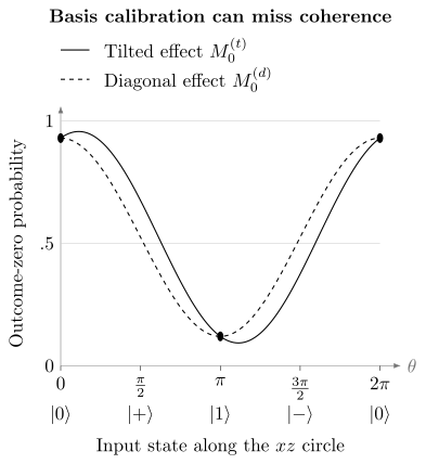
The same basis-state calibration supports both effects. Their predictions separate between the calibration states because one effect contains an off-diagonal matrix element. Additional trusted superposition probes can test this difference; the $xz$ circle shown here cannot determine an imaginary off-diagonal component.

Measurement tomography reconstructs effects from sufficiently informative trusted probes; detector tomography was demonstrated experimentally by Lundeen et al. (2009). A calibration performed only on basis states estimates diagonal entries, not the entire detector.

First outcomes do not determine repeated outcomes

An instrument supplies conditional maps $\mathcal I_y$ with effect $M_y=\mathcal I_y^\dagger(I)$. Compare

$$\begin{aligned} \mathcal L_y(\rho)&=\Pi_y\rho\Pi_y,\\ \mathcal J_y(\rho)&=\operatorname{Tr}(\Pi_y\rho)|+\rangle\langle+|. \end{aligned}$$

Both have the ideal $Z$ POVM. The first leaves the measured eigenstate; the second prepares $|+\rangle$ afterward. Given first outcome zero, a second ideal $Z$ measurement reports zero with probability one or one half. An assignment fidelity cannot determine this backaction or establish a nondemolition measurement.

Why a confusion table does not separate SPAM

Without an intervening process, calibration measures

$C_{y|x}=\operatorname{Tr}(M_y\rho_x).$

The command $x$ is not automatically the actual ideal outcome $z$. If preparation is a classical mixture with weights $B_{z|x}$ and measurement has response $A$, then

$C=AB.$

Already this restricted model has nonunique physical factorizations. For symmetric flips,

$$\begin{gathered} F(e)=\begin{pmatrix}1-e&e\\e&1-e\end{pmatrix},\\ F(a)F(b)=F(a+b-2ab). \end{gathered}$$

The table $F(0.18)$ can arise from perfect preparation and $18\%$ readout flips, from the reverse allocation, or from $10\%$ flips at each end. Another allocation is $F(0.05)F(13/90)$. All yield the same frequencies. Additional shots narrow uncertainty in $C$ without selecting a factorization.

State tomography uses calibrated measurement; detector tomography uses calibrated preparations; conventional process tomography uses both. Independent references, physical bounds or additional experiments can resolve some ambiguities, but their assumptions matter. For example, Lin et al. (2021) analyze SPAM separation using gate assumptions and an initially uncorrelated qubit, with bounds for imperfect gates. An unknown extra component does not become a trusted reference merely by being added to the circuit.

Self-consistent characterization and gauge freedom

Gate-set tomography fits preparation, measurement and operations jointly. In Liouville coordinates a sequence probability is

$p=\langle\!\langle M|G_L\cdots G_1|\rho\rangle\!\rangle.$

For an invertible coordinate transformation $S$, all such probabilities remain unchanged under

$$\begin{aligned} |\rho\rangle\!\rangle&\mapsto S|\rho\rangle\!\rangle,\\ G_j&\mapsto SG_jS^{-1},\\ \langle\!\langle M|&\mapsto\langle\!\langle M|S^{-1}. \end{aligned}$$

The adjacent factors cancel. Not every $S$ preserves physical states, effects and channels, so algebraic equivalence must not be confused with an arbitrary physical reassignment. Nevertheless, ambiguity can persist among fully physical models.

For example, suppose all intervening gates are unitary rotations, preparations have Bloch vectors $0.6\mathbf n_x$, and binary effects are $(I\pm0.8\mathbf m_s\cdot\boldsymbol\sigma)/2$. Replacing the preparation length by $0.8$ and the detector contrast by $0.6$ preserves every probability:

$p_+=\tfrac12[1+0.48\mathbf m_s\cdot R\mathbf n_x].$

Both descriptions are physical. Even arbitrary unitary sequences do not distinguish these two allocations. A genuinely trusted preparation or a further experiment with justified extra structure can do so. Nielsen et al. (2021) explains gauge freedom and practical gate-set tomography; device characterization gives the experimental methods.

Separate three questions: identifiability asks whether different parameters predict exactly the same data; conditioning asks how much uncertainty distinguishable parameters acquire; model adequacy asks whether the assumed model predicts the experiment at all. More shots address statistical uncertainty, not an exact gauge freedom or an omitted physical mechanism.

Correlations and drift in calibration

A shared fluctuating variable $\lambda$ can affect preparation and detection together. Then

$$\begin{gathered} \mathbb E_\lambda\operatorname{Tr}(M_{y,\lambda}\rho_{x,\lambda})\\ \ne\operatorname{Tr}(\overline M_y\,\overline\rho_x) \end{gathered}$$

in general. For an extreme example, half the runs prepare $|0\rangle$ with effect $M_0=|0\rangle\langle0|$, while the other half prepare $|1\rangle$ with $M_0=|1\rangle\langle1|$. Outcome zero always occurs. Averaging the state and effect separately gives $I/2$ and predicts probability $1/2$. Jackson and van Enk (2015) discuss tests for correlated SPAM.

For classical responses varying across epochs, the exact relation is

$$\begin{aligned} \overline{\mathbf q}&=\overline A\,\overline{\mathbf p}+\mathbf c,\\ \mathbf c&=\mathbb E[(A-\overline A)(\mathbf p-\overline{\mathbf p})]. \end{aligned}$$

Thus matching calibration and science epoch weights and keeping the science distribution fixed across epochs are sufficient for using the averaged response. They are not necessary: cancellation of the covariance term can also occur. Matching weights alone does not suffice when the prepared distribution changes with detector quality.

Acquire different commands in interleaved or randomized order, retain times and compare predictions on additional settings and later runs. This helps distinguish drift from command dependence; it does not make the device stationary (Proctor et al., 2020). Similarly, matching one-bit readout marginals does not establish a product multiqubit response. A simultaneous error can flip both bits together; exercise7 quantifies the resulting discrepancy.

Observed correlations can originate in preparation, gates, readout or postprocessing. Tests aimed at readout correlations need trusted product probes or explicit preparation bounds. Control and readout calibration discusses the detector hardware, and device characterization develops tests using varied settings and sequences.

Readout correction and its uncertainty

For binary response, let $\alpha=\Pr(y=1|z=0)$ and $\beta=\Pr(y=0|z=1)$. Then

$$A=\begin{pmatrix}1-\alpha&\beta\\\alpha&1-\beta\end{pmatrix}.$$

For $m=p_0-p_1$ and observed $u=q_0-q_1$,

$$\begin{aligned} u&=(\beta-\alpha)+(1-\alpha-\beta)m,\\ \widehat m&=\frac{\widehat u-\beta+\alpha}{1-\alpha-\beta}. \end{aligned}$$

Known calibration and $N$ independent shots give an unbiased estimator with

$\operatorname{Var}(\widehat m\mid A)=\frac{1-u^2}{N(1-\alpha-\beta)^2}.$

Invertibility requires $1-\alpha-\beta\ne0$, not positivity of this denominator. An anticorrelated detector can be relabeled. A small magnitude, however, magnifies sampling uncertainty. For symmetric error $e$ and true $p_0=0.7$, the following standard deviations of the corrected population use $N=10{,}000$ shots and exactly known calibration:

Error $e$	Observed $q_0$	Corrected standard deviation
$0.10$	$0.660$	$0.005921$
$0.49$	$0.504$	$0.249992$

Values are rounded to six decimals. At $e=1/2$ the detector is uninformative and cannot be inverted. The second row illustrates poor conditioning even though the response is formally invertible.

Estimated calibration adds uncertainty. For $d=1-\alpha-\beta$ and independent calibration covariance $\Sigma_{\alpha\beta}$, first-order propagation adds $\mathbf j^{\mathsf T}\Sigma_{\alpha\beta}\mathbf j$, where

$\mathbf j=\frac1d\begin{pmatrix}1+m\\m-1\end{pmatrix}.$

Shared data require cross-covariance terms. This linear approximation is unreliable when calibration fluctuations can approach the singular denominator. Clipping inverse estimates to physical probabilities changes the estimator and generally introduces bias; an inverse estimate outside $[0,1]$ is not a negative physical probability.

Correction changes an estimate under a model; it does not repair preparation, gates or measurement backaction. Correlated multiqubit response can also change the sampling cost (Bravyi et al., 2021). See measurement-error mitigation for constrained and observable-specific estimators. Likewise, fixed SPAM can enter randomized benchmarking as nuisance amplitude and offset under the standard stationary model; the fitted decay does not separately estimate preparation and readout errors (Magesan et al., 2012).

Exercises

1. Build an emitted-state channel

Show that $\mathcal R_\rho(A)=\operatorname{Tr}(A)\rho$ is CPTP for any finite input dimension, and construct a preparation with success probability $s$.

Solution

Write $\rho=\sum_a\lambda_a|a\rangle\langle a|$ and use input basis $|j\rangle$. The rectangular Kraus operators $K_{aj}=\sqrt{\lambda_a}|a\rangle\langle j|$ satisfy

$$\begin{aligned} \sum_{aj}K_{aj}AK_{aj}^\dagger&=\operatorname{Tr}(A)\rho,\\ \sum_{aj}K_{aj}^\dagger K_{aj}&=I_{\rm in}. \end{aligned}$$

Branches $s\mathcal R_\rho$ and $(1-s)\mathcal R_\tau$, for any density operator $\tau$ on the same output space, form a complete instrument. The successful output on a normalized input is $s\rho$; its conditional state is $\rho$ only for $s>0$. This example has input-independent success, whereas general preparation filters need not.

2. Reconstruct a coherent effect

Trusted inputs $|0\rangle,|1\rangle,|+\rangle,|+y\rangle=(|0\rangle+i|1\rangle)/\sqrt2$ give outcome-zero probabilities $0.93,0.12,0.675,0.445$. Find the effect and determine whether a binary assignment matrix can describe it on all states.

Solution

Write $M_0=\bigl(\begin{smallmatrix}a&b\\b^*&d\end{smallmatrix}\bigr)$. The first two inputs give $a=.93,d=.12$. The other probabilities are

$$\begin{aligned} p(0|+)&=(a+d)/2+\operatorname{Re}b,\\ p(0|+y)&=(a+d)/2-\operatorname{Im}b. \end{aligned}$$

Hence $b=.15+.08i$. The minus sign in the second equation follows from the stated $+y$ convention. The eigenvalues are approximately $0.085768$ and $0.964232$, so $\{M_0,I-M_0\}$ is a valid POVM. Its off-diagonal component rules out an exact classical assignment model in the computational basis, although the same basis-state table also fits a diagonal effect.

3. Compare repeated measurements

Give Kraus operators for the two instruments $\mathcal L_y$ and $\mathcal J_y$ above, and compute their conditional second-read distributions.

Solution

One Kraus operator per branch suffices: $L_y=|y\rangle\langle y|$ and $J_y=|+\rangle\langle y|$. Both have effect $|y\rangle\langle y|$, and each complete family has a trace-preserving sum. After outcome zero, the normalized states are $|0\rangle\langle0|$ and $|+\rangle\langle+|$. A second ideal $Z$ read gives distributions $(1,0)$ and $(1/2,1/2)$ respectively. Identical first outcomes therefore do not imply identical instruments.

4. Find equivalent physical descriptions

Check the three factorizations of $F(.18)$, and verify the Bloch-length example for an arbitrary sequence of unitary gates.

Solution

Multiplication gives $F(a)F(b)=F(a+b-2ab)$. The pairs $(a,b)=(0,.18),(.10,.10),(.05,13/90)$ all give $.18$; reversing either pair gives the same table. All factors are stochastic.

Unitary gates rotate Bloch vectors without changing their length. For state radius $r$ and detector contrast $\eta$, the probability is $(1+r\eta\mathbf m\cdot R\mathbf n)/2$. Both $(r,\eta)=(.6,.8)$ and $(.8,.6)$ give $r\eta=.48$. A Liouville scaling of the three Bloch coordinates by $4/3$ implements this change on the specified states and effects; it commutes with every unitary rotation. It is not a physical state map on the entire Bloch ball, which illustrates why a coordinate gauge need not itself be a quantum channel.

5. Include finite calibration statistics

Take $\alpha=.07$, $\beta=.12$, $m=.4$, $N=10{,}000$ science shots, and $5{,}000$ independent trusted basis-calibration shots per column. Find the leading standard deviation of corrected $m$.

Solution

Here $d=.81$ and $u=.374$. The science contribution to the variance is approximately $0.000131096$. Independent binomial calibration has variances $\alpha(1-\alpha)/5000$ and $\beta(1-\beta)/5000$. Contracting these with the squared derivatives $(1+m)^2/d^2$ and $(m-1)^2/d^2$ adds approximately $0.000050484$. The combined leading standard deviation is $0.013475$.

This is a first-order uncertainty estimate, not an exact assertion of unbiasedness after substituting random calibration into a ratio. It also assumes the basis probes themselves are known and the calibration applies to the science shots.

6. Test an averaged calibration

Two equally weighted epochs have symmetric readout errors $.02,.18$. First take science population $p_0=.75$ only in the second epoch. Then take equally weighted science epochs with populations $.9,.1$. Compare inversion using average error $.10$ with the desired population.

Solution

In the first case $q_0=.18+.64(.75)=.66$. Average-error inversion gives $(.66-.10)/.80=.70$, whereas the contemporaneous response recovers $.75$.

In the second case the observed probabilities are $.884$ and $.244$, averaging to $.564$. Despite matching epoch weights, average-response inversion gives $.58$, not the true average population $.50$. Here $\operatorname{Cov}(e,p_0)=-.032$, and the difference between averaged observed probability and the product-of-averages prediction is $-2\operatorname{Cov}(e,p_0)=.064$. Equal weights remove one confounding mechanism, not the correlation between detector quality and prepared distribution.

7. Compare correlated and independent readout flips

On a trusted $00$ probe, a detector flips both bits together with probability $.08$. Compare this with independent flips having the same marginal probabilities.

Solution

In order $(00,01,10,11)$, the correlated and product distributions are

$$\begin{aligned} \mathbf q_c&=(.92,0,0,.08)^{\mathsf T},\\ \mathbf q_p&=(.8464,.0736,.0736,.0064)^{\mathsf T}. \end{aligned}$$

Both have one-bit error $.08$, but their total-variation distance is $.1472$. The correlated error indicators have covariance $.08-.08^2=.0736$; the product covariance is zero. The parity-sign expectations are $1$ and $(1-2\times.08)^2=.7056$. Thus marginal calibration misses a substantial parity difference. Without trusted preparation or quantitative bounds, this experiment would reveal a discrepancy in the complete preparation–readout experiment rather than identify its physical cause.

References

• S. Bravyi, S. Sheldon, A. Kandala, D. C. McKay, and J. M. Gambetta, “Mitigating measurement errors in multiqubit experiments,” Physical Review A 103, 042605 (2021), doi:10.1103/PhysRevA.103.042605.
• C. Jackson and S. J. van Enk, “Detecting correlated errors in state-preparation-and-measurement tomography,” Physical Review A 92, 042312 (2015), doi:10.1103/PhysRevA.92.042312.
• J. Lin, J. J. Wallman, I. Hincks, and R. Laflamme, “Independent state and measurement characterization for quantum computers,” Physical Review Research 3, 033285 (2021), doi:10.1103/PhysRevResearch.3.033285.
• J. S. Lundeen, A. Feito, H. Coldenstrodt-Ronge, K. L. Pregnell, Ch. Silberhorn, T. C. Ralph, J. Eisert, M. B. Plenio, and I. A. Walmsley, “Tomography of quantum detectors,” Nature Physics 5, 27–30 (2009), doi:10.1038/nphys1133.
• F. B. Maciejewski, Z. Zimborás, and M. Oszmaniec, “Mitigation of readout noise in near-term quantum devices by classical post-processing based on detector tomography,” Quantum 4, 257 (2020), doi:10.22331/q-2020-04-24-257.
• E. Magesan, J. M. Gambetta, and J. Emerson, “Characterizing quantum gates via randomized benchmarking,” Physical Review A 85, 042311 (2012), doi:10.1103/PhysRevA.85.042311.
• E. Nielsen, J. K. Gamble, K. Rudinger, T. Scholten, K. Young, and R. Blume-Kohout, “Gate set tomography,” Quantum 5, 557 (2021), doi:10.22331/q-2021-10-05-557.
• T. Proctor, M. Revelle, E. Nielsen, K. Rudinger, D. Lobser, P. Maunz, R. Blume-Kohout, and K. Young, “Detecting and tracking drift in quantum information processors,” Nature Communications 11, 5396 (2020), doi:10.1038/s41467-020-19074-4.