Kraus, Choi, and Stinespring Views

Kraus operators, a Choi matrix and a Stinespring realization describe the same quantum channel from three useful perspectives: how to apply it, how to test it, and where information can go when an environment is included. Their common rank determines the smallest pure auxiliary space needed for an exact realization. It does not determine a physical bath’s size or a circuit’s cost.

We work in finite dimensions. Besides deterministic channels, we consider nonzero selected operations whose output trace is a success probability. The distinction matters whenever an environment is measured rather than discarded.

Helpful background. Quantum channels for QI introduces Kraus operators and the output–input Choi convention. Spectral decomposition supplies positive-matrix factorization, and partial trace explains the subsystem reductions below. The general representation theorems are developed in the open-systems volume.

One map, three realizations

Let $K_a$ be $d_{\rm out}\times d_{\rm in}$ matrices. They define

$$\Phi(A)=\sum_{a=1}^mK_aAK_a^\dagger.$$

For a channel, $\sum_aK_a^\dagger K_a=I$; for a selected operation it is $\preceq I$. Complete positivity alone does not distinguish these cases. For a state $\rho$, a selected output $\Phi(\rho)$ remains subnormalized until its trace has been saved as the event probability.

We use the unnormalized Choi operator

$$J_\Phi=\sum_{i,j}\Phi(|i\rangle\langle j|)\otimes|i\rangle\langle j|,$$

with output first, input second. Define

$$|K_a\rangle\!\rangle=\sum_{\mu,i}(K_a)_{\mu i} |\mu\rangle_{\rm out}|i\rangle_{\rm in}.$$

Flattening here orders entries as $(\mu,i)$, with input index fastest. It differs from column stacking, which puts the input factor first. This small ordering distinction matters for complex or rectangular matrices.

Choose an orthonormal auxiliary basis $\{|a\rangle_E\}$ and construct

$$V|\psi\rangle=\sum_aK_a|\psi\rangle\otimes|a\rangle_E.$$

The three descriptions then satisfy

$$\begin{aligned} J_\Phi&=\sum_a|K_a\rangle\!\rangle\langle\!\langle K_a|,\\ \Phi(\rho)&=\operatorname{Tr}_E(V\rho V^\dagger). \end{aligned}$$

The first expression is positive by construction. In the second, tracing the orthonormal environment states removes the cross terms and leaves the Kraus sum. Finally, $V^\dagger V=\sum_aK_a^\dagger K_a$: a channel gives an isometry, whereas a trace-nonincreasing operation gives a contraction. A contraction alone is not deterministic closed-system evolution. It describes a selected branch that must be accompanied by a failure branch in a full experiment. See the formal Kraus, Choi and Stinespring treatments for the general statements (Kraus; Choi; Stinespring; Watrous).

A matrix factor reveals the common rank

Put the flattened Kraus operators into columns:

$$A=\begin{bmatrix}|K_1\rangle\!\rangle&\cdots&|K_m\rangle\!\rangle\end{bmatrix}.$$

The two Gram matrices are

$$\begin{aligned} J&=AA^\dagger,\qquad G=A^\dagger A,\\ G_{ab}&=\operatorname{Tr}(K_a^\dagger K_b). \end{aligned}$$

They have the same nonzero eigenvalues: the squared singular values of $A$. Their sizes can differ, so their numbers of zero eigenvalues can differ. For a nonzero CP map,

$$r=\operatorname{rank}J=\operatorname{rank}A=\operatorname{rank}G$$

is the smallest exact Kraus-list length and the smallest auxiliary dimension in a pure-environment realization. A displayed list can be longer because its operators are dependent or zero. For the zero operation, the matrix rank is zero; it can be written with an empty Kraus sum, or a zero contraction using an ordinary nonzero-dimensional auxiliary space. The rank–dimension statement above avoids that degenerate convention issue.

If $J=\sum_{\alpha=1}^r\lambda_\alpha |v_\alpha\rangle\langle v_\alpha|$ with positive eigenvalues, a minimal family is obtained by reshaping $\sqrt{\lambda_\alpha}|v_\alpha\rangle$ in the stated output–input order. Degenerate eigenspaces can be rotated, and individual vectors can acquire phases. These changes alter the displayed operators but not the channel.

For a channel, $\operatorname{Tr}J=\operatorname{Tr}G=d_{\rm in}$. Neither $J$ nor $G$ is generally a normalized density operator. The trace-preserving condition is stronger than this scalar trace: it requires $\operatorname{Tr}_{\rm out}J=I_{\rm in}$.

The environment contains a complementary output

Tracing the system output instead of the environment gives

$$\widetilde\Phi(\rho) =\sum_{a,b}\operatorname{Tr}(K_b^\dagger K_a\rho) |a\rangle\langle b|_E.$$

This is the complementary channel for the chosen isometric realization. It is a quantum state, including coherences between the environment labels, not just a list of classical probabilities. For a selected contraction the same expression is subnormalized, with the selected event’s probability.

A purification explains the connection to $G$. Introduce a reference $R$ and the unnormalized vector $|\Omega\rangle=\sum_i|i\rangle|i\rangle$. Then

$$\begin{aligned} |\Gamma\rangle&=(V\otimes I_R)|\Omega\rangle\\ &=\sum_{a,\mu,i}(K_a)_{\mu i}|\mu\rangle_{ \rm out}|a\rangle_E|i\rangle_R. \end{aligned}$$

Its subsystem reductions, in this order, are

$$\operatorname{Tr}_E|\Gamma\rangle\langle\Gamma|=J, \qquad \operatorname{Tr}_{{\rm out},R}|\Gamma\rangle\langle\Gamma|=G^{\mathsf T}.$$

The transpose follows from the coefficient $\operatorname{Tr}(K_b^\dagger K_a)=G_{ba}$. For a channel, divide both reductions by $d_{\rm in}$ to obtain density operators. In particular, $\widetilde\Phi(I/d_{\rm in})=G^{\mathsf T}/d_{\rm in}$. The Schmidt rank of $|\Gamma\rangle$ across $({\rm out},R)\mid E$ is $r$, which explains the minimal auxiliary dimension.

Changing the Kraus family

Starting from a minimal family of length $r$, let $W$ be an $m\times r$ isometry, $W^\dagger W=I_r$, and set

$$L_b=\sum_aW_{ba}K_a.$$

Summing the unread branch maps gives the original channel because $\sum_bW_{ba}W_{bc}^*=\delta_{ac}$. For the column factors and dilations,

$$B=AW^{\mathsf T},\qquad V_L=(I_{\rm out}\otimes W)V_K.$$

The transpose in $B$ follows from mixing columns; it is not an adjoint. Two minimal realizations are related by an environment unitary. Longer lists are isometric embeddings of the same minimal space. Compare their Choi matrices or actions on an operator basis, not their first Kraus operators.

Complementary outputs transform as $\widetilde\Phi_L(\rho)=W\widetilde\Phi_K(\rho)W^\dagger$. With unrestricted coherent access to the auxiliary space, these isometric descriptions contain equivalent information about the input. A fixed measurement in the laboratory can nevertheless give different probabilities after that rotation. Distinguish changing coordinates, actively rotating the environment, and changing what is measured.

Worked example: dephasing with two environment measurements

Take $K_0=\sqrt{3/4}\,I$ and $K_1=\sqrt{1/4}\,Z$. The channel preserves populations and halves the off-diagonal entries. Its Choi eigenvalues are $3/2,1/2,0,0$, so a two-dimensional auxiliary space is minimal. For an input with Bloch component $r_z$, its complementary output is

$$\widetilde\Phi(\rho)= \begin{pmatrix}3/4&\sqrt3\,r_z/4\\ \sqrt3\,r_z/4&1/4\end{pmatrix}.$$

The diagonals do not depend on $r_z$, but the off-diagonal entry does. This information becomes visible in a different measurement basis:

Environment measurement	Branch operators	Probabilities
computational basis	$K_0,K_1$	$3/4,\ 1/4$
Hadamard basis	$L_\pm=(K_0\pm K_1)/\sqrt2$	$p_\pm=1/2\pm\sqrt3\,r_z/4$

For $\boldsymbol r=(1/5,-2/5,3/5)$, the second probabilities are $1/2\pm3\sqrt3/20$. In either measurement, discarding the outcome gives the same system output with Bloch vector $(1/10,-1/5,3/5)$. An instrument contains the outcome-dependent operations, so these are different instruments sharing one unread channel.

More generally, measuring an orthonormal environment basis $|\mu\rangle$ produces $L_\mu={}_E\langle\mu|V$. General measurements and coarse-grained outcomes can require several operators per outcome. A spectral Kraus decomposition alone does not show that any such measurement occurred, or define a time-resolved physical trajectory.

Worked example: reset transfers information

The reset channel is

$$\begin{aligned} \mathcal R(\rho)&=|0\rangle\langle0|\operatorname{Tr}\rho,\\ K_0&=|0\rangle\langle0|,\quad K_1=|0\rangle\langle1|. \end{aligned}$$

Its Choi operator is $\operatorname{diag}(1,1,0,0)$ and has rank two. The associated isometry is particularly simple:

$$V|\psi\rangle=|0\rangle_S|\psi\rangle_E.$$

One realization swaps the input qubit with an auxiliary qubit prepared in $|0\rangle$. The system output is fixed, while the complementary output is exactly $\rho$. If the input was entangled with a reference, those correlations move to the auxiliary qubit as well; they have not been destroyed by a global unitary.

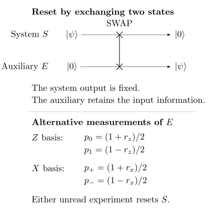
Reset from the system’s perspective is information transfer in this pure auxiliary realization. Measuring $E$ in the $Z$ or $X$ basis gives different classical records; these are alternative experiments. Discarding either record leaves the system in $|0\rangle$.

For the input used above, measuring $E$ in the computational basis gives probabilities $(4/5,1/5)$, while its Hadamard-basis measurement gives $(3/5,2/5)$. Both instruments leave the system reset. The choice of accessible environment and measurement must be specified before asking what information an observer receives.

Exact compression and approximate truncation

Composing channels with Kraus lists $\{K_a\}$ and $\{L_b\}$ produces operators $L_bK_a$. Their number is only an upper bound on the resulting Choi rank. For two dephasing channels with probabilities $1/4$ and $1/3$, the four products are proportional to $I,Z,Z,I$, with squared coefficients

$$\frac12,\quad\frac16,\quad\frac14,\quad\frac1{12}.$$

Combining like directions gives the exact two-operator family $\{\sqrt{7/12}\,I,\sqrt{5/12}\,Z\}$. No approximation was made.

Dropping a nonzero Choi eigenmode is different. For a channel with exact positive $J$, retaining only some spectral terms gives a CP, trace- nonincreasing map, because the omitted part is itself CP. It generally fails to preserve trace. If the omitted Kraus operators are $D_a$, define

$$F_{\rm drop}=\sum_aD_a^\dagger D_a.$$

The lost probability on input $\rho$ is $\operatorname{Tr}(F_{\rm drop}\rho)$, with maximum $\|F_{\rm drop}\|_\infty$. This is a direct physical measure of the truncation, unlike an unexplained numerical rank threshold. Renormalizing each surviving output can make a nonlinear conditional rule, not a repaired channel. If a new trace-preserving approximation is needed, construct it explicitly and compare its predictions with the original.

Numerical work must still check Hermiticity, eigenvalue tolerances and trace conditions: inaccurate factorization is not the same as exact spectral truncation. Compare degenerate subspaces rather than arbitrary eigenvector phases. The channel-coordinate example gives a compact executable check using complete matrix-unit action.

Minimal dimension does not determine the physical environment

Choi rank gives the smallest auxiliary dimension for an exact pure realization. A mixed laboratory environment can be purified by adding another system; which systems are actually accessible is a separate question. A low Choi rank neither identifies the bath nor guarantees an inexpensive circuit. State preparation, interactions, routing, reset and approximation accuracy all affect implementation cost.

Nor does a one-use realization specify what happens on reuse. Resetting the environment between uses and retaining it produce different multitime experiments. Initial correlations and restricted preparation procedures can also prevent a common channel from describing every input. These questions require the appropriate open-system model and memory analysis, rather than another Kraus-basis change. Formal continuity results compare nearby channels through suitable dilations, but do not by themselves give a hardware synthesis cost (Kretschmann, Schlingemann and Werner).

Exercises

1. Truncate an amplitude-damping channel

Let $K_0=\operatorname{diag}(1,\sqrt{1-\gamma})$ and $K_1=\sqrt\gamma|0\rangle\langle1|$, with $0<\gamma<1$. These are orthogonal spectral Kraus directions. If $K_1$ is dropped, find the trace deficit on an arbitrary input and its maximum. Show explicitly that normalizing the retained output need not preserve mixtures.

Solution

$F_{\rm drop}=\gamma|1\rangle\langle1|$, so the deficit is $\gamma\rho_{11}\leq\gamma$. The retained operation is CP-TNI, not TP. Its normalized outputs on $|0\rangle$ and $|1\rangle$ are those same pure states. However, the normalized output on their equal mixture is

$$\frac{\operatorname{diag}(1,1-\gamma)}{2-\gamma},$$

which is not $I/2$. At $\gamma=1/2$ it is $\operatorname{diag}(2/3,1/3)$. Conditioning has changed the mixing weights.

2. Compare the Choi and Kraus Gram spectra

For a rectangular Kraus-column matrix $A$, prove that $AA^\dagger$ and $A^\dagger A$ have the same nonzero spectrum, and deduce the common minimal dimension.

Solution

If $A^\dagger Ay=\lambda y$ with $\lambda>0$, then $Ay\ne0$ and $AA^\dagger(Ay)=\lambda(Ay)$. Conversely, $AA^\dagger x=\lambda x$ implies that $A^\dagger x\ne0$ is a $\lambda$ eigenvector of $A^\dagger A$. The maps preserve multiplicities on every positive eigenspace, equivalently giving the squared nonzero singular values of $A$. Hence $\operatorname{rank}(AA^\dagger)=\operatorname{rank}A=\operatorname{rank}(A^\dagger A)=r$. Exactly $r$ independent Kraus columns are necessary and sufficient, and the Schmidt form of the associated purification needs exactly $r$ environment dimensions.

3. Rotate a dephasing instrument

Apply the Hadamard label rotation to the dephasing family and derive the branch probabilities for an input with Bloch component $r_z$. Explain the physical limitation.

Solution

$L_\pm=(K_0\pm K_1)/\sqrt2$ and $\sum_\pm L_\pm\rho L_\pm^\dagger=\sum_aK_a\rho K_a^\dagger$. Moreover, $L_\pm^\dagger L_\pm=I/2\pm(\sqrt3/4)Z$, so $p_\pm=1/2\pm\sqrt3 r_z/4$. At $r_z=3/5$ these become $1/2\pm3\sqrt3/20$. Both effects sum to $I$, rechecking completeness. The rotated and unrotated branch families are different instruments with one unread channel; neither label is a physical detector event unless a corresponding environment measurement has been specified.

4. Compress two composed dephasing maps

Compose dephasing probabilities $p_1=1/4$ and $p_2=1/3$, compress the four products, and check exact rank and TP.

Solution

The two $I$ products have squared weights $(1-p_1)(1-p_2)+p_1p_2=1/2+1/12=7/12$. The two $Z$ products have total weight $(1-p_1)p_2+p_1(1-p_2)=1/4+1/6=5/12$. Thus the minimal family is $\{\sqrt{7/12}I,\sqrt{5/12}Z\}$. Its completeness sum is $I$, its Choi eigenvalues are $7/6$ and $5/6$, and its exact rank is two. The original count four is only a redundant list length; numerical compression would additionally declare a tolerance and recheck TP after truncation.

5. Align minimal and padded realizations

Pad a minimal pair $\{K_0,K_1\}$ to $\{K_0/\sqrt2,K_0/\sqrt2,K_1\}$ and exhibit the environment embedding.

Solution

Use

$$W=\begin{pmatrix}1/\sqrt2&0\\1/\sqrt2&0\\0&1\end{pmatrix}, \qquad W^\dagger W=I_2.$$

Then $L_b=\sum_aW_{ba}K_a$ gives the padded triple, $B=AW^{\mathsf T}$, and $BB^\dagger=AA^\dagger$. The corresponding dilation is $V_L=(I\otimes W)V_K$; its environment is three-dimensional but its occupied support and minimal dimension remain two. A second padded realization must first be embedded in the same ambient space before a unitary alignment is sought. Removing any nonzero direction would require new TP and action checks.

6. Retain and measure the reset environment

For the reset isometry, find the complementary output and the computational- and Hadamard-basis branch probabilities on the worked input with Bloch vector $(1/5,-2/5,3/5)$.

Solution

$V\lvert\psi\rangle=\lvert0\rangle\lvert\psi\rangle$, so tracing the system gives $\widetilde{\mathcal R}(\rho)=\rho$, while tracing $E$ gives $\lvert0\rangle\!\langle0\rvert$. Computational measurement uses $K_0,K_1$ and reads the diagonal probabilities $(4/5,1/5)$. Hadamard measurement uses $(K_0\pm K_1)/\sqrt2$ and reads $(1\pm r_x)/2=(3/5,2/5)$. In each basis the subnormalized branch maps sum to $\mathcal R$ and their traces sum to one. These outcomes describe the specified environment measurements, not a unique trajectory inherent in the reset channel.

References

• M.-D. Choi, “Completely Positive Linear Maps on Complex Matrices,” Linear Algebra and its Applications 10, 285–290 (1975), doi:10.1016/0024-3795(75)90075-0.
• K. Kraus, “General State Changes in Quantum Theory,” Annals of Physics 64, 311–335 (1971), doi:10.1016/0003-4916(71)90108-4.
• K. Kraus, States, Effects, and Operations: Fundamental Notions of Quantum Theory, Lecture Notes in Physics 190, Springer-Verlag, Berlin (1983), doi:10.1007/3-540-12732-1.
• D. Kretschmann, D. Schlingemann, and R. F. Werner, “The Information-Disturbance Tradeoff and the Continuity of Stinespring’s Representation,” IEEE Transactions on Information Theory 54, 1708–1717 (2008), doi:10.1109/TIT.2008.917696.
• W. F. Stinespring, “Positive Functions on C*-Algebras,” Proceedings of the American Mathematical Society 6, 211–216 (1955), doi:10.1090/S0002-9939-1955-0069403-4.
• J. Watrous, The Theory of Quantum Information, Cambridge University Press, Cambridge (2018), doi:10.1017/9781316848142.