Common Noise Models

A noise model predicts how a quantum state changes during a specified operation or time interval. The same reported “error probability” can describe different maps, and maps with the same average fidelity can give different circuit outcomes. This page compares common qubit models through their action on populations and coherences, then explains which assumptions permit their repeated use.

Helpful background. Density operators provide the matrix entries used below; quantum channels explain complete positivity and trace preservation. For microscopic derivations and Kraus constructions, see common noise channels.

Pauli mixtures and depolarizing conventions

A stochastic Pauli channel on $n$ qubits is

$$\begin{aligned} \mathcal E(\rho)&=\sum_{P\in\mathcal P_n}p_P P\rho P,\\ p_P&\geq0,\qquad\sum_Pp_P=1, \end{aligned}$$

where $\mathcal P_n$ contains one representative of each Pauli string, without global phases. Each term is a possible unitary fault. The map is unital, $\mathcal E(I)=I$, and diagonal in the Pauli operator basis. This makes stabilizer propagation particularly simple. Neither independence across qubits nor independence across time follows from this formula.

For a qubit, compare two depolarizing conventions:

$$\begin{aligned} \mathcal D_q^{\mathrm{rep}}(\rho) &=(1-q)\rho+qI/2,\\ \mathcal D_p^{\mathrm P}(\rho) &=(1-p)\rho +\frac p3(X\rho X+Y\rho Y+Z\rho Z). \end{aligned}$$

The first has a literal replacement interpretation for $0\leq q\leq1$; the second is a probability mixture for $0\leq p\leq1$. Their common Bloch-vector action is $\mathbf r\mapsto\lambda\mathbf r$, with

$$\lambda=1-q=1-\frac{4p}{3}, \qquad q=\frac{4p}{3}.$$

Thus $p>3/4$ still gives a valid Pauli channel, but its $q>1$ is no longer a replacement probability. At $p=1$, the Bloch vector reverses and shrinks by $1/3$; this is not the impossible perfect universal spin flip.

For the identity target, average infidelity is

$r=1-F_{\mathrm{avg}}=q/2=2p/3.$

These are three different error parameters, not interchangeable labels. Translate through the channel action before transferring a value between a paper and a simulator. The depolarizing-channel derivation gives the higher-dimensional complete-positivity range.

Coherence loss and coherent phase

In a chosen basis, a population-preserving qubit channel has

$$\begin{aligned} \rho_{00}'&=\rho_{00},\qquad\rho_{11}'=\rho_{11},\\ \rho_{01}'&=\lambda\rho_{01},\qquad |\lambda|\leq1. \end{aligned}$$

Hermiticity fixes $\rho_{10}'=(\rho_{01}')^*$. Writing $\lambda=|\lambda|e^{-i\theta}$ separates coherence attenuation from a $Z$ rotation through $\theta$. For real $\lambda$, the equivalent phase-flip mixture has

$p_Z=(1-\lambda)/2.$

An API might instead define a phase-damping strength $g$ by $\lambda=\sqrt{1-g}$. Only with that definition does $g=1-\lambda^2$ hold. The basis also matters: dephasing preserves energy populations only when its preferred basis is the energy basis.

A fixed overrotation $V_\epsilon=e^{-i\epsilon Z/2}$ has $\lambda=e^{-i\epsilon}$ and loses no purity. Averaging unobserved angles instead gives

$\lambda=\mathbb E[e^{-i\epsilon}].$

The argument of this complex average determines the residual rotation. The mean angle alone does not: equal probabilities for $\epsilon=0$ and $2\pi$ have mean $\pi$ but give the identity channel. Conversely, asymmetric zero-mean angle distributions can give a complex $\lambda$.

How angles are sampled matters on repeated use. A slowly varying angle shared by many gates and a freshly sampled angle at every gate can have the same one-step channel but different later behavior; the explicit comparison shows this distinction. Randomized compiling can produce effective Pauli noise under specified assumptions, but that description belongs to the randomized ensemble, not automatically to the original circuit (Wallman and Emerson, 2016).

Relaxation and the Bloch-ball center

Zero-temperature amplitude damping transfers population from $|1\rangle$ to $|0\rangle$:

$$\begin{aligned} \rho_{00}'&=\rho_{00}+\gamma\rho_{11},\\ \rho_{11}'&=(1-\gamma)\rho_{11},\\ \rho_{01}'&=\sqrt{1-\gamma}\,\rho_{01},\qquad0\leq\gamma\leq1. \end{aligned}$$

Its Bloch action is

$$\begin{pmatrix}x\\y\\z\end{pmatrix}\mapsto \begin{pmatrix} \sqrt{1-\gamma}x\\ \sqrt{1-\gamma}y\\ (1-\gamma)z+\gamma \end{pmatrix}.$$

The translation moves the maximally mixed state toward the ground state. A Pauli channel has no such translation, so matching one fidelity number cannot reproduce this behavior.

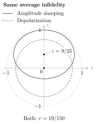
Equal average infidelity does not imply equal noise. Amplitude damping with $\gamma=9/25$ maps the unit circle to an ellipse centered at $z=9/25$; depolarization with shrink factor $56/75$ gives a concentric circle. Both have $r=19/150$. The solid ellipse still touches the ground state at $z=1$, while the dashed circle contracts every pure state.

For constant downward and upward rates $\Gamma_\downarrow,\Gamma_\uparrow\geq0$, let $\Gamma=\Gamma_\downarrow+\Gamma_\uparrow>0$. In the phase-covariant Markov model, with coherent precession removed,

$$\begin{aligned} n_{\mathrm{eq}}&=\Gamma_\uparrow/\Gamma,\qquad \gamma_T=1-e^{-\Gamma\Delta t},\\ \rho_{11}'&=(1-\gamma_T)\rho_{11}+\gamma_T n_{\mathrm{eq}},\\ \rho_{01}'&=\sqrt{1-\gamma_T}\,\rho_{01}. \end{aligned}$$

Both rates zero give the identity map; no unique equilibrium population is then selected. Rates have units of inverse time. For a thermal bath with level spacing $\hbar\omega$, detailed balance gives $\Gamma_\uparrow/\Gamma_\downarrow=e^{-\beta\hbar\omega}$. A fitted fixed population alone does not establish a thermal bath.

The zero-temperature limit is $n_{\mathrm{eq}}=0$. For an exponential relaxation time $T_1=1/\Gamma$, the population contraction is $e^{-\Delta t/T_1}$. Relaxation already attenuates coherence by $e^{-\Delta t/(2T_1)}$. To match an exponential $T_2$, add only

$$\lambda_\phi=e^{-\Delta t/T_\phi},\qquad \frac1{T_\phi}=\frac1{T_2}-\frac1{2T_1}.$$

The combined coherence factor is $e^{-\Delta t/T_2}$. Adding a separate dephasing factor already equal to $e^{-\Delta t/T_2}$ counts the relaxation contribution twice. Nonnegative pure-dephasing rate requires $T_2\leq2T_1$ within this model. Ramsey, echo, driven and nonexponential decay measurements need not supply interchangeable parameters; see dephasing and amplitude damping.

Erasure requires more than a visible flag

The standard erasure channel has an isometric surviving branch and an orthogonal failure flag. Its linear action on any input operator $A$ is

$$\mathcal E_\epsilon(A) =(1-\epsilon)VAV^\dagger +\epsilon\operatorname{Tr}(A)|e\rangle\langle e|,$$

where $V^\dagger V=I$, $|e\rangle$ is orthogonal to the range of $V$, and $0\leq\epsilon\leq1$. The flag probability is input-independent, and successful transmission preserves the state up to $V$ (Bennett, DiVincenzo, and Smolin, 1997).

A detectable loss need not have either property. For example, let the surviving filter be $K=\operatorname{diag}(1,1/2)$ and the loss operator be $L=(\sqrt3/2)|e\rangle\langle1|$. Then $K^\dagger K+L^\dagger L=I$, but survival probabilities are $1$ for $|0\rangle$ and $1/4$ for $|1\rangle$. On $|+\rangle$,

$$\begin{aligned} p_{\mathrm{surv}}&=5/8,\\ |\psi_{\mathrm{surv}}\rangle&=(2|0\rangle+|1\rangle)/\sqrt5. \end{aligned}$$

The flag locates a failure, but the surviving state is also filtered. Replacing this process by a constant-probability erasure channel would miss that distortion. Erasure and loss channels also distinguishes flagged loss from bosonic attenuation, detector inefficiency and postselection.

Leakage populations and their limits

Leakage leaves a computational subspace $\mathcal H_C$ for $\mathcal H_L$ inside a larger physical space. Write $Q_C,Q_L$ for the projectors and $p_C,p_L$ for their populations. A two-state population model uses

$$\begin{gathered} \begin{pmatrix}p_C'\\p_L'\end{pmatrix} =\begin{pmatrix}1-\ell&s\\\ell&1-s\end{pmatrix} \begin{pmatrix}p_C\\p_L\end{pmatrix},\\ 0\leq\ell,s\leq1. \end{gathered}$$

Here $\ell$ is leakage per step and $s$ is return, or seepage. This is an exact closed population equation for every physical input only if the full channel satisfies

$\Phi^\dagger(Q_L)=\ell Q_C+(1-s)Q_L.$

Indeed, taking its expectation in any input gives precisely the second row above. The condition rules out dependence on the state within either sector and on coherence between sectors. For a qutrit with $\mathcal H_C=\operatorname{span}\{|0\rangle,|1\rangle\}$, coherent coupling only between $|1\rangle$ and $|2\rangle$ violates it: $|0\rangle$ never leaks, whereas $|1\rangle$ does. An averaged population approximation can still be useful, but requires specifying how states are averaged or randomized (Wood and Gambetta, 2018).

For $\ell+s>0$, the stationary population and exact repeated-step solution are

$$\begin{aligned} p_L^*&=\frac{\ell}{\ell+s},\\ p_L(m)&=p_L^*+[p_L(0)-p_L^*](1-\ell-s)^m. \end{aligned}$$

Convergence from every initial population requires $0<\ell+s<2$. At $\ell=s=1$, populations alternate; the stationary value $1/2$ is generally not a long-time limit. At $\ell=s=0$, every population is stationary. Even when leakage vanishes, the model says nothing about errors within $\mathcal H_C$, and return from leakage need not restore the encoded state. See leakage and crosstalk for the full-space description.

Joint faults and circuit placement

For two qubits with only $X$ faults, assign probabilities

$$\begin{gathered} p_{XI}=p_1,\quad p_{IX}=p_2,\quad p_{XX}=p_c,\\ p_{II}=1-p_1-p_2-p_c, \end{gathered}$$

all nonnegative. The marginal fault probabilities are $q_1=p_1+p_c$ and $q_2=p_2+p_c$. Independence holds exactly when

$p_c=q_1q_2.$

A nonzero $XX$ probability alone therefore does not establish a correlated fault model: independent faults can occur simultaneously. The allowed joint range at fixed marginals is

$\max(0,q_1+q_2-1)\leq p_c\leq\min(q_1,q_2).$

Quantum correlations need not arise from Pauli mixtures. A shared fluctuating field generates $e^{-i\theta(Z_1+Z_2)/2}$; the subspace spanned by $|01\rangle,|10\rangle$ is unaffected, unlike under independent phase fluctuations. Temporal correlations likewise require more than a one-step map; zero covariance at a lag does not prove statistical independence.

Placement matters even without memory. On input $|0\rangle$, applying $X$ and then amplitude damping gives $\gamma|0\rangle\langle0|+(1-\gamma)|1\rangle\langle1|$. Damping first and then applying $X$ gives the pure state $|1\rangle$. A gate-local product of fitted channels additionally assumes that environmental memory does not correlate the intervals. Markovian and non-Markovian noise explains that requirement.

Choose the simplest model that predicts measurements not used in fitting. This small set of tests distinguishes several otherwise similar models:

Test	Structure it can reveal
Prepare the three Bloch axes	Isotropy versus a preferred dephasing or relaxation axis
Prepare the maximally mixed state	Nonunital drift, invisible to a Pauli model
Vary depth and echo sequence	Coherent accumulation and temporal memory
Compare isolated and simultaneous operations	Context dependence and joint faults
Resolve loss and test surviving states	A standard erasure map versus state-dependent filtering

Preparation and measurement errors can also change these observations. Include them explicitly rather than attributing every discrepancy to gate noise.

Exercises

1. Convert depolarizing conventions

A simulator uses replacement probability $q=0.012$. Find the total nonidentity Pauli probability $p$, Bloch shrink factor $\lambda$, and average infidelity $r$.

Solution

$p=3q/4=0.009$, $\lambda=1-q=0.988$, and $r=q/2=0.006$. All four values describe the same channel, but each answers a different question.

2. Translate dephasing parameters

Coherences are multiplied by $\lambda=0.94$. Find the equivalent phase-flip probability and the strength $g$ of an API defined by $\lambda=\sqrt{1-g}$. Does a nonzero mean random angle necessarily imply a nonzero average rotation?

Solution

$p_Z=(1-0.94)/2=0.03$, whereas $g=1-0.94^2=0.1164$. The channel action determines which conversion applies. For the last question, equal probabilities for angles $0$ and $2\pi$ have nonzero mean but $\mathbb E[e^{-i\epsilon}]=1$: both unitary conjugations are the identity.

3. Build a matched T1–T2 idle model

Let $T_1=100\,\mu\mathrm{s}$, exponential $T_2=80\,\mu\mathrm{s}$, and $\Delta t=1\,\mu\mathrm{s}$. Compute $T_\phi$, damping probability $\gamma$, and additional coherence factor $\lambda_\phi$.

Solution

$$\begin{aligned} T_\phi^{-1}&=(1/80-1/200)\,\mu\mathrm{s}^{-1},\\ T_\phi&=(400/3)\,\mu\mathrm{s},\\ \gamma&=1-e^{-1/100}\simeq0.009950,\\ \lambda_\phi&=e^{-3/400}\simeq0.992528. \end{aligned}$$

The combined coherence factor is $e^{-1/200}e^{-3/400}=e^{-1/80}\simeq0.987578$, as required.

4. Find a thermal fixed point

Take $\Gamma_\uparrow=10^3\,\mathrm{s}^{-1}$ and $\Gamma_\downarrow=9\times10^3\,\mathrm{s}^{-1}$. Find the fixed excited population and its value after $100\,\mu\mathrm{s}$ from the ground state.

Solution

The fixed value is $n_{\mathrm{eq}}=0.1$. Since $\Gamma\Delta t=1$, the final excited population is $0.1(1-e^{-1})\simeq0.063212$. Zero-temperature amplitude damping would incorrectly leave the ground state unchanged. These are transition rates, not angular frequencies: no factor of $2\pi$ belongs in the exponent.

5. Analyze leakage and seepage

Let $\ell=0.002$, $s=0.05$, and $p_L(0)=0$. Find the one-cycle population and long-time limit. Then examine $\ell=s=1$ with the same initial state.

Solution

One cycle gives $p_L(1)=0.002$. Here $1-\ell-s=0.948$, so

$p_L(m)=\frac1{26}(1-0.948^m)\longrightarrow\frac1{26}\simeq0.038462.$

The larger limiting population reflects repeated leakage and slow return. For $\ell=s=1$, $p_L(m)=[1-(-1)^m]/2$: it alternates between zero and one. Solving a stationary equation alone would not detect this failure to converge.

6. Detect a correlated Pauli fault

Let $p_{II}=0.97$ and $p_{XI}=p_{IX}=p_{XX}=0.01$. Find both marginals and compare the joint $XX$ probability with independence.

Solution

Both marginals are $q_1=q_2=0.02$. Independence predicts $p_{XX}=0.02^2=0.0004$, whereas the actual value is $0.01$, twenty-five times larger. For comparison, the distribution $(0.9604,0.0196,0.0196,0.0004)$ has exactly the same marginals and is independent despite its nonzero $XX$ term.

7. Distinguish models with equal fidelity

Verify that the two channels in the figure have the same average infidelity, using $F_{\mathrm{avg}}=1/2+\operatorname{Tr}(T)/6$ for the qubit affine map $\mathbf r\mapsto T\mathbf r+\mathbf t$. Give an input and measurement that distinguish them. How would you separate $Z$ dephasing from a fixed $Z$ overrotation?

Solution

Damping has $T=\operatorname{diag}(4/5,4/5,16/25)$, hence $\operatorname{Tr}T=56/25$. Depolarization has $T=(56/75)I$, with the same trace. Thus $F_{\mathrm{avg}}=131/150$ and $r=19/150$.

Prepare $I/2$ and measure $Z$: damping gives expectation $9/25$, depolarization zero. To probe phase noise, prepare $|+\rangle$ and measure both $X$ and $Y$ at several depths. Fixed overrotation produces signed rotating quadratures; real positive dephasing contracts them without rotation. Computational-basis survival alone does not distinguish those two processes.

References

• C. H. Bennett, D. P. DiVincenzo, and J. A. Smolin, “Capacities of quantum erasure channels,” Physical Review Letters 78, 3217–3220 (1997), doi:10.1103/PhysRevLett.78.3217.
• H.-P. Breuer and F. Petruccione, The Theory of Open Quantum Systems, Oxford University Press, 2002, doi:10.1093/acprof:oso/9780199213900.001.0001.
• M. A. Nielsen and I. L. Chuang, Quantum Computation and Quantum Information, 10th anniversary edition, Cambridge University Press, 2010, doi:10.1017/CBO9780511976667.
• J. J. Wallman and J. Emerson, “Noise tailoring for scalable quantum computation via randomized compiling,” Physical Review A 94, 052325 (2016), doi:10.1103/PhysRevA.94.052325.
• C. J. Wood and J. M. Gambetta, “Quantification and characterization of leakage errors,” Physical Review A 97, 032306 (2018), doi:10.1103/PhysRevA.97.032306.