Symmetry Verification

Symmetry verification uses a property that the ideal answer must satisfy—such as a fixed parity or particle number—to reject incompatible outcomes or estimate a projected observable. It can remove some errors without identifying their cause. Errors that stay inside the accepted sector remain, and the loss of samples can offset an improvement in accuracy.

The starting point is a specific ideal state $\rho_\star$ and a projector $\Pi$ satisfying $\Pi\rho_\star\Pi=\rho_\star$. The state, check and observable matter: a symmetry of the Hamiltonian does not by itself imply that the prepared state lies in one symmetry sector. This page develops direct and virtual projection, imperfect checks, finite-sample uncertainty and several limits of filtering.

Required background. Projectors explains orthogonal subspaces. Error mitigation introduces bias, variance and sampling cost.

Helpful background. Good quantum numbers explains conserved eigenspaces. Variance and covariance supplies uncertainty propagation.

The accepted symmetry sector

For a Hermitian binary symmetry $S$ with $S^2=I$, the projector onto eigenvalue $s=\pm1$ is

$\Pi_s=\frac{I+sS}{2}.$

Because $S^2=I$, $\Pi_s^2=\Pi_s$; Hermiticity follows from $S^\dagger=S$. The ideal input and dynamics determine the intended sign. Choosing whichever sign produces a favorable measured answer would select a different target.

For example, the odd-parity subspace of two qubits is spanned by $|01\rangle,|10\rangle$ and has $S=Z\otimes Z=-1$. A single $X$ fault flips parity. A $Z$ fault preserves parity and may still destroy coherence between those basis states. Two parity-changing faults can return the state to the accepted sector.

More generally, an error $E$ anticommuting with $S$ maps an $s$ eigenstate into the $-s$ sector. Commuting errors remain undetected by that check. Detection probabilities depend on the full circuit, timing and noise model, as in the simulation studies of Bonet-Monroig et al. (2018) and McArdle, Yuan and Benjamin (2019).

The ideal complete circuit must preserve the promised support at the point of verification. Requiring every gate to commute with $S$ is sufficient but stronger than necessary. If the algorithm intentionally mixes sectors, or an approximation breaks the symmetry, filtering can remove valid signal. A particle-number check can use its full spectral projector rather than only parity; degeneracy preserves the whole eigenspace.

What an ideal projection changes

For the actual noisy state $\rho$, let

$$\begin{aligned} a&=\operatorname{Tr}(\Pi\rho),\\ \rho_\Pi&=\frac{\Pi\rho\Pi}{a},\qquad a>0. \end{aligned}$$

Here $a$ is the acceptance probability. An ideal selective Lüders measurement actually prepares $\rho_\Pi$ on acceptance. Its mean for any observable is

$\mu_\Pi=\frac{\operatorname{Tr}(O\Pi\rho\Pi)}a.$

If $[O,\Pi]=0$, this reduces to $\operatorname{Tr}(O\Pi\rho)/a$. In a compatible terminal measurement it is the conditional mean of $O$ among accepted records. Without commutation, the one-sided shortcut is generally wrong and may even be complex. An actual sequential measurement, or a suitable correlation protocol, is needed for the two-sided expression. See Lüders measurements.

Fidelity can improve while an observable gets worse

For a pure ideal target $|\psi_\star\rangle$ inside the sector, define squared fidelity $F=\langle\psi_\star|\rho|\psi_\star\rangle$. Ideal projection gives

$F_\Pi=F/a\geq F.$

This follows by moving $\Pi$ onto the target ket and bra. It is a statement about an ideal projector and this target fidelity, not every observable or an imperfect checking circuit.

Consider three orthogonal states labeled $0,1,2$, ideal state $|0\rangle$, and

$$\begin{aligned} \Pi&=\operatorname{diag}(1,1,0),\\ \rho&=\operatorname{diag}(.8,.1,.1),\\ O&=\operatorname{diag}(0,1,-1). \end{aligned}$$

The ideal and raw means of $O$ are both zero. Projection improves fidelity from $.8$ to $8/9$, but changes the mean to $1/9$. The rejected sector’s contribution had accidentally canceled the in-sector error. High acceptance is also not fidelity: $|1\rangle$ passes this check with certainty but is orthogonal to the target.

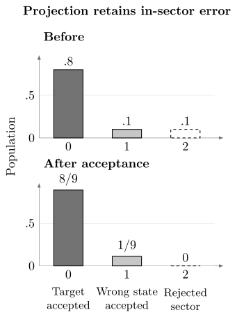
Projection removes state $2$ and renormalizes states $0$ and $1$. Target population increases, but the remaining population of state $1$ produces observable error $1/9$. The bars describe an ideal check, so this limitation does not require detector mistakes.

Direct checks and virtual projection

A terminal bitstring can reveal parity or particle number without extra gates if it also supports the desired observable measurement. A nondemolition ancilla check can preserve coherence inside the accepted subspace before another measurement, but its extra gates and backaction may add noise. The check’s success probability alone does not characterize that backaction.

Virtual symmetry verification estimates the projected mean from correlations, without necessarily preparing the projected state. For binary $S$ and $[O,S]=0$,

$\mu_s=\frac{\langle O\rangle+s\langle OS\rangle}{1+s\langle S\rangle}.$

This is the exact identity obtained by substituting $\Pi_s$. The measurements of $O,S,OS$ may share records or use different settings, so their covariance and shot allocation matter. The direct-versus-correlation distinction is discussed by Bonet-Monroig et al. (2018) and Huggins et al. (2021).

As an example, take compatible joint outcomes:

$S$	$O$	Probability
$+1$	$+1$	$.54$
$+1$	$-1$	$.18$
$-1$	$+1$	$.08$
$-1$	$-1$	$.20$

Then $\langle O\rangle=.24$, $\langle S\rangle=.44$ and $\langle OS\rangle=.48$. For the positive sector, $a=.72$, the unnormalized moment is $.36$, and the conditional mean is $.50$. Those three values describe different quantities.

Symmetry expansion replaces the exact projector by a chosen weighted combination $\Gamma$ of symmetry operations (Cai, 2021). A quotient such as $\operatorname{Tr}(O\Gamma\rho)/\operatorname{Tr}(\Gamma\rho)$ can trade bias against sampling cost. It need not describe a physical postselected state when $\Gamma$ is not a suitable positive projector. That broader construction should be distinguished from ordinary sector filtering.

Multiple checks and correlations

For commuting Hermitian involutions $S_j$, multiply their projectors:

$\Pi_{\boldsymbol s}=\prod_j\frac{I+s_jS_j}{2}.$

For two checks, this is

$$\Pi_{s_1,s_2}=\tfrac14\bigl[I+s_1S_1+s_2S_2 +s_1s_2S_1S_2\bigr].$$

Both acceptance and the projected numerator contain the cross term. Commuting observables do not imply statistically independent outcomes. For example, the following joint law gives marginal acceptances $.70,.71$ but joint acceptance $.56$:

$(S_1,S_2)$	Probability with $O=+1$	Probability with $O=-1$
$(+,+)$	$.42$	$.14$
$(+,-)$	$.08$	$.06$
$(-,+)$	$.10$	$.05$
$(-,-)$	$.06$	$.09$

The acceptance covariance is $.56-(.70)(.71)=.063$. The jointly accepted mean is $(.42-.14)/.56=.5$. Getting $6000$ accepted records therefore takes about $10714$ attempts on average under independent stationary trials; multiplying marginal rates would incorrectly predict about $12072$.

Redundant generators impose no new subspace restriction when their target signs are consistent. For instance, adding $S_3=S_1S_2$ with $s_3=s_1s_2$ leaves the projector unchanged; an inconsistent sign makes the joint sector empty. Extra measured checks can still reveal measurement faults, but their outcomes cannot be counted as independent passes.

For a finite Abelian symmetry group, the projector for character $\chi$ is $|G|^{-1}\sum_g\chi(g)^*U_g$, using each group element once. Expanding this average can require many correlations; compatible grouping or randomized group sampling changes the measurement cost, not the operator identity.

If projectors $P,Q$ do not commute, $QP$ is generally not a projector onto their common subspace. Sequential acceptance implements $\rho\mapsto QP\rho PQ$ and can depend on order. An orthogonal projector onto a common eigenspace, when that space exists, is a separate construction.

Sampling cost and ratio uncertainty

Write estimated numerator and acceptance as $\widehat n,\widehat a$, with population ratio $\mu=n/a$. Abbreviate their variances and covariance as

$$\begin{aligned} V_n&=\operatorname{Var}(\widehat n),\\ V_a&=\operatorname{Var}(\widehat a),\\ C_{na}&=\operatorname{Cov}(\widehat n,\widehat a). \end{aligned}$$

To leading order,

$$\operatorname{Var}(\widehat\mu) \simeq\frac{V_n+\mu^2V_a-2\mu C_{na}}{a^2}.$$

The leading ratio bias is

$$\mathbb E\widehat\mu-\mu \simeq\frac{\mu V_a-C_{na}}{a^2}.$$

These are local approximations; a poorly resolved denominator can make them unreliable. In the first probability table, define $A=1$ for $S=+1$ and zero otherwise. The single-shot quantities satisfy

$$\begin{aligned} \operatorname{Var}(AO)&=.5904,\\ \operatorname{Var}(A)&=.2016,\\ \operatorname{Cov}(AO,A)&=.1008. \end{aligned}$$

For $N=20000$ independent attempts, the ratio formula gives variance about $5.2083\times10^{-5}$ and standard error $.007217$. Omitting covariance would overestimate this example’s variance. Other measurement designs can have a different sign or magnitude of covariance.

Exact counting for direct postselection

With independent identically distributed records, fixed decision rule and acceptance $a$, the retained count is $K\sim\operatorname{Binomial}(N,a)$. Conditional on $K>0$, the retained sample mean is exactly unbiased for the accepted population. If its single-record variance is $\sigma_A^2$, then

$$\begin{aligned} \Pr(K=0)&=(1-a)^N,\\ \operatorname{Var}(\widehat\mu\mid K>0) &=\sigma_A^2\mathbb E[1/K\mid K>0]. \end{aligned}$$

The familiar $\sigma_A^2/(Na)$ is a large-count approximation, not the exact result. An empty accepted sample has no sample mean and should not be reported as zero. Stopping at a fixed $M$ accepted records instead gives variance $\sigma_A^2/M$ and expected attempts $M/a$, under the same independent-trial assumptions.

Correlation estimates measured in separate settings generally form a different ratio estimator. Their numerator and denominator variances need not shrink with $a$, leading to an $a^{-2}$ amplification; direct selection often has an $a^{-1}$ leading cost. Neither is a universal overhead independent of measurement grouping, covariance or the observable.

Imperfect acceptance and measurement disturbance

Suppose a classical sector label is well defined in the acquisition. Let $\pi$ be its valid-sector prevalence, $\alpha$ the true-accept probability, and $\beta$ the false-accept probability. If selection is independent of the observable within each sector, then

$$\begin{aligned} a_{\rm obs}&=\alpha\pi+\beta(1-\pi),\\ n_{\rm obs}&=\alpha\pi\mu_{\rm in}+\beta(1-\pi)\mu_{\rm out},\\ \mu_{\rm obs}&=n_{\rm obs}/a_{\rm obs}. \end{aligned}$$

For $(\pi,\alpha,\beta)=(.75,.92,.10)$ and sector means $(.4,-.6)$, acceptance is $.715$, the accepted mean is about $.3650$, and invalid records form about $3.50\%$ of the accepted sample. False rejection occurs on $.06$ of all attempts. Collecting $5000$ accepted records costs about $6993$ attempts on average.

Two average assignment rates are insufficient if acceptance depends on the observable or on the state inside a sector. They also do not describe disturbance by a physical check. For example, Kraus operator $U\Pi$, with $U$ unitary inside the accepted subspace, has exactly the same acceptance effect $\Pi$ as a Lüders check but rotates the accepted state. A check can have perfect sector labels and still damage the desired observable. Calibrate the appropriate joint measurement or instrument, including leakage and loss classes.

Combining filtering with other mitigation

When readout errors can change both the observable and the sector label, keep their joint outcome counts. Measurement-error mitigation can then estimate the required projected moments under its response assumptions. Discarding rejected records first can remove information needed for that correction, although identifiability must be assessed for the particular response and target rather than assumed impossible in every reduced model.

Zero-noise extrapolation of a conditional ratio differs from extrapolating numerator and denominator before division. With probabilistic error cancellation weights $w_i$, a projected ratio uses both signed sums:

$\widehat\mu=\frac{\sum_iw_iA_iO_i}{\sum_iw_iA_i}.$

The denominator is a signed estimate, not an ordinary retained fraction. Keep its covariance with the numerator and separately count actual accepted and rejected attempts. Under exact PEC and a guaranteed ideal sector, the ideal denominator is already one; the unbiased weighted numerator can be used directly. Dividing by an estimated denominator produces a different, generally biased finite-sample estimator, even if both have the same infinite-data limit.

Choose checks and tuning on data separate from the final comparison, test their transfer to representative circuits and observables, and compare accuracy at equal total resources. Physical selective projection can improve a state, while virtual estimation changes only the reported expectation. Neither alone supplies the general logical recovery conditions of quantum error correction.

Exercises

1. Derive binary virtual projection

Prove that $(I+sS)/2$ is a projector and derive the virtual mean when $[O,S]=0$.

Solution

Squaring gives $(I+2sS+S^2)/4=(I+sS)/2$. Hermiticity follows from $S^\dagger=S$. The numerator is $(\langle O\rangle+s\langle OS\rangle)/2$, and acceptance is $(1+s\langle S\rangle)/2$. Their ratio yields the stated formula whenever acceptance is positive.

2. Reconstruct the two-check moments

Use the second table to compute $\langle S_1\rangle$, $\langle S_2\rangle$, $\langle S_1S_2\rangle$ and their three $O$-weighted counterparts. Recover joint acceptance and numerator from the projector expansion.

Solution

The symmetry moments are $(.40,.42,.42)$; $\langle O\rangle=.32$ and the weighted moments are $(.28,.34,.18)$. Thus acceptance is $(1+.40+.42+.42)/4=.56$, and numerator is $(.32+.28+.34+.18)/4=.28$. Their ratio is $.5$. The cross terms cannot be replaced by products of marginal means.

3. Quantify false-accept contamination

Reproduce the imperfect-check example and its bias relative to the true valid-sector mean.

Solution

Valid accepted mass is $.92(.75)=.69$ and invalid accepted mass is $.1(.25)=.025$. The numerator is $.69(.4)+.025(-.6)=.261$. Dividing by $.715$ gives about $.3650$, with bias $-.03497$. Equivalently, the contamination fraction $.025/.715$ multiplies the sector-mean difference $-.6-.4=-1$.

4. Compute exact conditional variance

For $N$ independent attempts with acceptance $a$ and accepted-record variance $\sigma_A^2$, express the exact variance given that at least one record is accepted. Explain why a fixed-accepted-count experiment differs.

Solution

Condition on $K=k$: the mean has variance $\sigma_A^2/k$ and the same expectation $\mu$ for every $k>0$. Averaging gives

$\frac{\sigma_A^2}{1-(1-a)^N}\sum_{k=1}^{N}\frac1k\binom Nk a^k(1-a)^{N-k}.$

There is no between-$K$ variance of the conditional mean because its expectation is constant. Stopping at $M$ accepted records fixes the variance to $\sigma_A^2/M$ and randomizes the attempt count instead.

5. Test the one-sided shortcut

Take $\Pi=|0\rangle\langle0|$, $\rho=|+\rangle\langle+|$ and $O=X$. Compare the one-sided quotient and the Lüders mean. What happens for $O=Y$?

Solution

Acceptance is $1/2$. For $X$, the one-sided quotient is one, but the projected state is $|0\rangle$, with $X$ mean zero. For the standard $Y$ matrix, the one-sided quotient is $i$, while the projected $Y$ mean is again zero. Incompatible one-sided products are not generally physical conditional means.

6. Reverse two noncommuting checks

Start in $|0\rangle$. Compare accepting first $P=|0\rangle\langle0|$, then $Q=|+\rangle\langle+|$, with the reverse order.

Solution

The first order accepts with probability $1(1/2)=1/2$ and leaves $|+\rangle$. The reverse accepts with probability $(1/2)(1/2)=1/4$ and leaves $|0\rangle$. These are sequential instruments. Their common one-dimensional eigenspaces do not intersect, so neither sequence realizes an orthogonal projection onto a shared nonzero subspace.

7. Explain the population figure

Compute acceptance, target fidelity and observable mean before and after projection in the three-state example. Does the ideal-sector promise ensure an improvement in every observable?

Solution

Acceptance is $.9$. The normalized populations are $(8/9,1/9,0)$, so target fidelity rises from $.8$ to $8/9$. The raw observable mean $.1-.1=0$ equals its ideal value, whereas the projected mean is $1/9$. Thus the fidelity guarantee is compatible with a worse individual observable.

8. Separate correct labels from a correct instrument

In the same three-state space, let $U$ swap states $0,1$ and preserve state $2$. Compare accepted Kraus operators $K=\Pi$ and $K'=U\Pi$ on the ideal input $|0\rangle$.

Solution

Both have effect $K^\dagger K=K'^\dagger K'=\Pi$, so acceptance is one and sector labels are identical. The first outputs $|0\rangle$ and the second $|1\rangle$, changing target fidelity from one to zero and the example’s observable from zero to one. A sector confusion matrix alone cannot distinguish these instruments.

References

• X. Bonet-Monroig, R. Sagastizabal, M. Singh, and T. E. O’Brien, “Low-Cost Error Mitigation by Symmetry Verification,” Physical Review A 98, 062339 (2018), doi:10.1103/PhysRevA.98.062339.
• Z. Cai, “Quantum Error Mitigation Using Symmetry Expansion,” Quantum 5, 548 (2021), doi:10.22331/q-2021-09-21-548.
• W. J. Huggins, J. R. McClean, N. C. Rubin, Z. Jiang, N. Wiebe, K. B. Whaley, and R. Babbush, “Efficient and Noise Resilient Measurements for Quantum Chemistry on Near-Term Quantum Computers,” npj Quantum Information 7, 23 (2021), doi:10.1038/s41534-020-00341-7.
• S. McArdle, X. Yuan, and S. Benjamin, “Error-Mitigated Digital Quantum Simulation,” Physical Review Letters 122, 180501 (2019), doi:10.1103/PhysRevLett.122.180501.